Note

Click here to download the full example code

Samples and support¶

Geostatistics starts from measurements taken at known places. Before you compute a statistic, you need to know where each value was taken and how much rock it represents. This chapter follows samples from the drill hole to the block and measures, on real data, how the volume behind a value changes its statistics.

import sys
from pathlib import Path

HERE = Path(__file__).parent if "__file__" in globals() else Path.cwd()
sys.path.insert(0, str(HERE.parents[1] / "examples"))

What you'll learn

What a sample is: a value, a location and a volume.
How boitatá holds samples, drill holes and grids, and how it marks missing values.
How a drill hole goes from collar and survey to coordinates, and why assays are composited.
The volume-variance effect: larger supports keep the mean and lose variance.
Why preferential sampling biases the plain mean.

Prerequisites: basic Python and NumPy. No geostatistics.

What a sample is¶

A sample is a measured value at a location. Walker Lake, the first dataset in this chapter, holds 470 samples of a variable V in ppm over a 260 × 300 m area. Each sample has an easting, a northing and a value.

A sample also has a volume, and that volume is easy to forget. A soil sample weighs a few hundred grams. A length of drill core holds a few kilograms. A block in a mine plan holds thousands of tonnes. Geostatisticians call the volume a value stands for its support (Figure 1).

Figure 1. Three supports. The same number, say 2 % zinc, can describe a point, a 2 m length of core or a block of ground.

Key idea

Report every grade with its support. Grades on different supports have different distributions, even when they come from the same rock, so compare them only after bringing them to one support.

Coordinates and containers¶

Samples live in boitatá's own containers: PointSet for scattered samples, Drillholes for holes with intervals, and BlockModel for grids of blocks. Each container stores the geometry once (coordinates, a grid definition, a rotation) and the variables as named columns. The columns are Apache Arrow arrays, so a container hands them to NumPy, polars or pandas without copying. Algorithms read the geometry from the container, so you pass it once.

bt.datasets.walker_lake() downloads the samples once, caches them, and returns a PointSet:

import boitata as bt
import matplotlib.pyplot as plt
import numpy as np
from common import ACCENT, GRAY, HIGHLIGHT, LIGHT, map_axes, save

samples = bt.datasets.walker_lake()
print(samples)
print(samples.coords[:3])
print(samples["V"][:3])

Out:

PointSet(470 points, crs: none)
  ID: Float64
  V: Float64
  U: Float64
  T: Float64
[[11.  8.  0.]
 [ 8. 30.  0.]
 [ 9. 48.  0.]]
[  0.    0.  224.4]

coords is an (n, 3) array. Walker Lake is a map, so boitatá pads the missing elevation with z = 0: every algorithm works in 3D, and a 2D dataset is a flat 3D one. Indexing by name returns a column as a NumPy array.

Not every sample has every variable. A missing value is an Arrow null, never a sentinel number such as -999 that could slip into an average. NumPy shows nulls as NaN; polars counts them:

u = samples["U"]
print(f"U measured at {np.count_nonzero(~np.isnan(u))} of {len(samples)} samples")
print(samples.to_polars().null_count().row(0, named=True))

Out:

U measured at 275 of 470 samples
{'x': 0, 'y': 0, 'z': 0, 'ID': 0, 'V': 0, 'U': 195, 'T': 0}

U was measured at 275 of the 470 samples; the other 195 are null. Statistics and estimators in boitatá skip nulls, and the file readers turn the usual sentinels (-999, -99, 1e21) into nulls on the way in.

A BlockModel describes a grid by its corner, its block size and its block count, and computes the block centers when asked. A 20 m grid over Walker Lake has 13 × 15 blocks:

grid = bt.BlockModel(origin=(0.5, 0.5), size=(20, 20), count=(13, 15))
print(grid)
print(grid.coords[:2])

Out:

BlockModel(regular, 195 of 195 cells, count [13, 15, 1], size [20.0, 20.0, 1.0], rotation [0.0, 0.0, 0.0])
[[10.5 10.5  0.5]
 [30.5 10.5  0.5]]

Drill holes¶

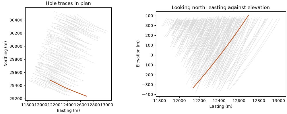
Most samples in mining come from drill holes. Three tables describe a drill hole (Figure 2):

the collar: where the hole starts, as x, y, z;
the survey: the direction of the hole, measured at stations down the hole as depth, dip and azimuth;
the intervals: what was measured between two depths, FROM and TO, such as an assay grade or a rock type.

Figure 2. A drill hole in section. The collar fixes the start, the survey stations give the direction at each depth, and desurveying turns any depth into coordinates. Holes often flatten as they deepen.

A drill hole bends. Desurveying reconstructs its path from the collar through each survey station, so any depth down the hole has coordinates. The stacked sulphide lenses dataset has 289 holes:

data = bt.datasets.stacked_sulphide_lenses()
collars, surveys, assays, lithology = data["collars"], data["surveys"], data["assays"], data["lithology"]
print(f"{collars.num_rows} collars, {surveys.num_rows} survey stations, {assays.num_rows} assays")
hole = "DD0027"  # @param {type:"string"}
row = np.flatnonzero(collars["HOLE_ID"] == hole)[0]
print(f"collar: X {collars['X'][row]:.1f}  Y {collars['Y'][row]:.1f}  Z {collars['Z'][row]:.1f}")
for i in np.flatnonzero(surveys["HOLE_ID"] == hole)[[0, 1, 2, -1]]:
    print(
        f"survey at {surveys['DEPTH'][i]:5.1f} m: dip {surveys['DIP'][i]:.1f}, azimuth {surveys['AZIMUTH'][i]:.1f}"
    )

Out:

289 collars, 4348 survey stations, 16995 assays
collar: X 12696.7  Y 29235.4  Z 403.5
survey at   0.0 m: dip 55.2, azimuth 289.9
survey at  30.0 m: dip 54.7, azimuth 290.8
survey at  60.0 m: dip 54.4, azimuth 289.9
survey at 958.1 m: dip 45.7, azimuth 296.3

Hole DD0027 leaves the collar dipping 55.2° toward azimuth 289.9° (west-northwest) and ends, 958.1 m down, at 45.7° toward 296.3°. Drillholes desurveys every hole when you build it. merge_intervals first combines the assay and lithology tables so that each interval carries its grades and its rock type; at returns the coordinates of any depth:

holes = bt.Drillholes(collars, surveys, bt.merge_intervals(assays, lithology))
paths = holes.paths()
print(holes)
top, bottom = holes.at([hole, hole], [0.0, 900.0])
print(f"{hole}: collar at {top.round(1)}, 900 m down at {bottom.round(1)}")
print(f"offset from the collar: {(bottom - top).round(1)}")

fig, (a, b) = plt.subplots(1, 2, figsize=(10, 4), layout="constrained")
ids = paths["HOLE_ID"]
for ax, (i, j) in ((a, ("x", "y")), (b, ("x", "z"))):
    for h in np.unique(ids):
        keep = ids == h
        ax.plot(paths[i][keep], paths[j][keep], color=LIGHT, lw=0.6)
    keep = ids == hole
    ax.plot(paths[i][keep], paths[j][keep], color=HIGHLIGHT, lw=1.8)
    ax.set_aspect("equal")
map_axes(a, "Hole traces in plan")
b.set(title="Looking north: easting against elevation", xlabel="Easting (m)", ylabel="Elevation (m)")
save(fig, "holes")

Hole traces in plan, Looking north: easting against elevation

Out:

Drillholes(289 holes, 17848 intervals)
  HOLE_ID: Utf8
  FROM: Float64
  TO: Float64
  ZN_PCT: Float64
  PB_PCT: Float64
  CU_PCT: Float64
  AG_GPT: Float64
  AU_GPT: Float64
  DENSITY: Float64
  LITH: Utf8
DD0027: collar at [12696.7 29235.4   403.5], 900 m down at [12174.  29463.9  -290.9]
offset from the collar: [-522.7  228.5 -694.4]

At 900 m down the hole, DD0027 sits 522.7 m west, 228.5 m north and 694.4 m below its collar. The orange trace in both views is this hole; the gray ones are the other 288.

Compositing¶

Assays come in whatever lengths the geologist chose to split the core. Here the lengths run from 0.25 m to 2.75 m, and 97 % lie within 0.1 m of 1 m or 2 m. A 0.25 m assay and a 2.75 m assay have different supports, so their values do not share one distribution. Compositing combines the assays into intervals of one length, so every value represents the same volume (Figure 3).

Figure 3. Compositing to 2 m. Each composite grade is the average of the assays it covers, weighted by sampled length. The composites stop at the contact, and core that was never sampled counts as missing, not as zero. The metal, grade × length, is the same before and after.

Two rules keep compositing honest. A composite never averages across a geological contact, because the grades on each side belong to different populations. Unsampled core stays missing: reading it as zero dilutes the grade. composite(2.0, ..., domain="LITH") applies both rules and returns a PointSet of composites located at their midpoints.

length = assays["TO"] - assays["FROM"]
print(f"assay lengths: median {np.median(length):.2f} m, from {length.min():.2f} to {length.max():.2f} m")
near = np.minimum(np.abs(length - 1), np.abs(length - 2)) <= 0.1
print(f"{near.mean():.0%} of the assays lie within 0.1 m of 1 m or 2 m")
composites = holes.composite(2.0, ["ZN_PCT"], domain="LITH")
print(f"{len(composites)} composites of 2 m")
metal_assays = np.sum(assays["ZN_PCT"] * length)
metal_composites = np.sum(composites["ZN_PCT"] * composites["ZN_PCT_length"])
print(f"Zn metal: assays {metal_assays:.1f}, composites {metal_composites:.1f}")
assert abs(metal_composites / metal_assays - 1) < 1e-9

Out:

assay lengths: median 1.97 m, from 0.25 to 2.75 m
97% of the assays lie within 0.1 m of 1 m or 2 m
13602 composites of 2 m
Zn metal: assays 15710.3, composites 15710.3

The 16 995 assays become 13 602 composites of 2 m. Keep the final check in any compositing script: zinc metal, grade × sampled length summed over all intervals, is 15 710.3 before and after. Compositing moves metal between intervals; it must not create or lose any.

Pitfall

Weighting a composite by its full length instead of its sampled length reads unsampled core as zero grade. The mean drops and metal vanishes. Use the <grade>_length column that composite returns, as in the metal check above.

Support and the volume-variance effect¶

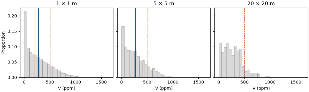
Average values over larger volumes and the mean stays the same, because the blocks together hold the same values. The variance falls, because averaging cancels highs against lows: the larger the support, the narrower the histogram. This is the volume-variance effect (Figure 4).

Figure 4. Walker Lake V averaged over 1, 5 and 20 m blocks. The mean stays at 278 ppm; the variance and the share of values above 500 ppm both fall as the blocks grow.

Start down the holes. Composite the massive sulphide (MS) zone at 1, 2, 4 and 8 m and compare the zinc grades, weighting each composite by its sampled length:

print(f"{'length':>7}{'n':>7}{'mean':>8}{'variance':>10}")
for size in (1.0, 2.0, 4.0, 8.0):
    c = holes.composite(size, ["ZN_PCT"], domain="LITH")
    ms = c["LITH"] == "MS"
    stats = bt.describe(c["ZN_PCT"][ms], weights=c["ZN_PCT_length"][ms])
    print(f"{size:>6.0f}m{ms.sum():>7}{stats['mean']:>8.2f}{stats['variance']:>10.1f}")

Out:

 length      n    mean  variance
     1m   1202    8.93      29.9
     2m    627    8.93      24.4
     4m    339    8.93      20.1
     8m    197    8.93      16.1

The mean zinc grade stays at 8.93 % for every length. The variance falls from 29.9 %² at 1 m to 16.1 %² at 8 m.

Walker Lake lets you watch the same effect in two dimensions, with the truth in hand. Besides the 470 samples, the dataset has an exhaustive grid: 78 000 values, one per square meter. row_at returns the block each value falls in, and np.bincount averages the values per block:

exhaustive = bt.datasets.walker_lake_exhaustive()
points = np.c_[exhaustive["X"], exhaustive["Y"]]
print(f"{'block':>6}{'blocks':>8}{'mean':>7}{'variance':>10}{'> 500 ppm':>11}")
blocks = {}
for size in (1, 5, 10, 20):
    grid = bt.BlockModel(origin=(0.5, 0.5), size=(size, size), count=(260 // size, 300 // size))
    rows = grid.row_at(points)
    v = np.bincount(rows, weights=exhaustive["V"]) / np.bincount(rows)
    blocks[size] = v
    print(f"{size:>4} m{len(v):>8}{v.mean():>7.0f}{v.var():>10.0f}{(v > 500).mean():>11.1%}")

fig, axes = plt.subplots(1, 3, figsize=(10, 3), layout="constrained", sharey=True)
bins = np.linspace(0, 1650, 34)
for ax, size in zip(axes, (1, 5, 20), strict=True):
    v = blocks[size]
    ax.hist(v, bins, weights=np.full(len(v), 1 / len(v)), color=LIGHT, edgecolor=GRAY, lw=0.5)
    ax.axvline(v.mean(), color=ACCENT, lw=1.4)
    ax.axvline(500, color=HIGHLIGHT, lw=1, ls="--")
    ax.set(title=f"{size} × {size} m", xlabel="V (ppm)")
axes[0].set_ylabel("Proportion")
save(fig, "support")

1 × 1 m, 5 × 5 m, 20 × 20 m

Out:

 block  blocks   mean  variance  > 500 ppm
   1 m   78000    278     62422      18.8%
   5 m    3120    278     52287      16.7%
  10 m     780    278     46694      16.2%
  20 m     195    278     37617      11.3%

Every block size gives a mean of 278 ppm. The variance falls from 62 422 ppm² for 1 m cells to 37 617 ppm² for 20 m blocks, and the histogram loses its spike near zero and its tail above 1000 ppm.

The last column matters most to a mine. Suppose rock above 500 ppm is ore. On 1 m cells, 18.8 % of the area is ore; on 20 m blocks, 11.3 % is. A mine that selects ore in 20 m blocks cannot recover the 18.8 % that the small-scale data suggest. A resource estimate must therefore state its support. Chapters 4 and 5 return to this: kriging estimates block averages, and simulation lets you average to any support you choose.

The math

The average of \(n\) independent values with variance \(\sigma^2\) has variance \(\sigma^2 / n\). Grades are not independent: nearby values resemble each other, so averaging cancels less than \(1/n\) would suggest. The variance of blocks \(v\) within a deposit \(A\) is [ D^2(v \mid A) = D^2(\cdot \mid A) - \bar\gamma(v, v), ] the point variance minus \(\bar\gamma(v, v)\), the average variogram between two points drawn inside one block. The variogram, which measures how values differ with distance, is the subject of chapter 3.

Pitfall

Statistics on different supports do not mix. Do not compare the histogram of 1 m assays with that of a 20 m block model and call the difference a bias: part of it is the volume-variance effect.

Preferential sampling¶

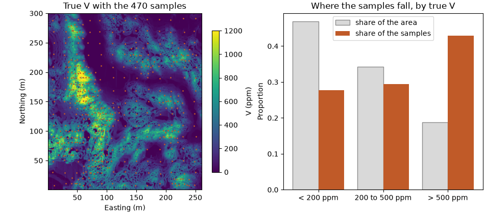
Samples are rarely spread evenly. Geologists drill a first campaign on a regular grid, find the rich zones, and drill those more densely to define them (Figure 5). The data then over-represent high grades.

Figure 5. Preferential sampling. Infill holes cluster in the rich zone, so a small part of the area holds most of the samples.

Walker Lake was sampled this way. With the exhaustive grid you can compare where the samples fall with what the area holds:

at_samples = exhaustive["V"].reshape(300, 260)[samples.y.astype(int) - 1, samples.x.astype(int) - 1]
print(f"samples: mean V {samples['V'].mean():.0f} ppm; whole area: {exhaustive['V'].mean():.0f} ppm")
classes = ["< 200", "200 to 500", "> 500"]
edges = [0, 200, 500, np.inf]
area = np.histogram(exhaustive["V"], edges)[0] / len(exhaustive["V"])
sampled = np.histogram(at_samples, edges)[0] / len(samples)
for name, x, y in zip(classes, area, sampled, strict=True):
    print(f"true V {name:>10} ppm: {x:6.1%} of the area, {y:6.1%} of the samples")

fig, (a, b) = plt.subplots(1, 2, figsize=(9.5, 4.2), layout="constrained")
image = a.imshow(
    exhaustive["V"].reshape(300, 260), origin="lower", extent=(0.5, 260.5, 0.5, 300.5), vmin=0, vmax=1200
)
a.scatter(*samples.coords[:, :2].T, s=4, color=HIGHLIGHT, linewidths=0)
map_axes(a, "True V with the 470 samples")
fig.colorbar(image, ax=a, shrink=0.8, label="V (ppm)")
position = np.arange(3)
b.bar(position - 0.2, area, 0.4, color=LIGHT, edgecolor=GRAY, label="share of the area")
b.bar(position + 0.2, sampled, 0.4, color=HIGHLIGHT, label="share of the samples")
b.set_xticks(position, [f"{c} ppm" for c in classes])
b.set(title="Where the samples fall, by true V", ylabel="Proportion")
b.legend()
save(fig, "clustering")

True V with the 470 samples, Where the samples fall, by true V

Out:

samples: mean V 435 ppm; whole area: 278 ppm
true V      < 200 ppm:  46.9% of the area,  27.7% of the samples
true V 200 to 500 ppm:  34.3% of the area,  29.4% of the samples
true V      > 500 ppm:  18.8% of the area,  43.0% of the samples

Ground above 500 ppm covers 18.8 % of the area but holds 43.0 % of the samples. The plain mean of the samples, 435 ppm, overstates the true mean of 278 ppm by more than half. Declustering corrects this by giving each sample a weight in proportion to the area it represents; chapter 2 shows how.

Check before you move on

A grade of 2 % in a 1 m assay and a grade of 2 % in a 20 m block describe different volumes. Which of the two histograms do you expect to be wider?
Why must a composite not cross a lithology contact?
What does boitatá store for an assay that was never taken, and why not -999?
After compositing, which quantity must match the assays exactly?
43.0 % of the Walker Lake samples sit on ground above 500 ppm. Why does that not mean 43 % of the area is ore?