unfolding¶

Unfold flattens a layer that undulates between two surfaces. it gives each point coordinates in the frame of the layer: w from 0 on the footwall to 1 on the hanging wall, and (u, v) along it. variograms and kriging then run on the unfolded coordinates, and the estimates go back to the real blocks row by row. the layer here is the saprolite of a nickel laterite, between the bedrock and the limonite above it.

import sys
from pathlib import Path

HERE = Path(__file__).parent if "__file__" in globals() else Path.cwd()
sys.path.insert(0, str(HERE.parents[1]))

import boitata as bt
import matplotlib.pyplot as plt
import numpy as np
from common import ACCENT, GRAY, HIGHLIGHT, INK, save

the bounding surfaces¶

448 vertical holes log four horizons from the top: ferricrete (FERR), limonite (LIM), saprolite (SAP) and bedrock (BRK). the base of the saprolite is the bedrock contact, and its top the limonite contact. both are gridded on 10 m cells: the bedrock elevation and the saprolite thickness by inverse distance, the top as their sum, so the surfaces never cross. grid_surface turns each grid into a mesh.

data = bt.datasets.nickel_laterite_profile()
horizons = data["horizons"]
holes = bt.Drillholes.from_tables(data, intervals=None)
sap = horizons["HORIZON"] == "SAP"
ids = list(horizons["HOLE_ID"][sap])
top, base = horizons["FROM"][sap], horizons["TO"][sap]
contact = holes.at(ids, base)

grid = bt.BlockModel(origin=(29975, 59975, 0), size=(10, 10, 1), count=(106, 76, 1))
idw = bt.InverseDistance(bt.Search(radius=150, max_samples=12, min_samples=3))
bedrock_z = idw.fit(contact[:, :2], contact[:, 2]).predict(grid)
thickness = idw.fit(contact[:, :2], base - top).predict(grid)
bedrock = bt.grid_surface(grid.with_column("z", bedrock_z), "z")
limonite = bt.grid_surface(grid.with_column("z", bedrock_z + thickness), "z")
print(bedrock)
print(
    f"bedrock {np.nanmin(bedrock_z):.0f} to {np.nanmax(bedrock_z):.0f} m, "
    f"saprolite {np.nanmin(thickness):.1f} to {np.nanmax(thickness):.1f} m thick"
)

Out:

Mesh(8056 vertices, 15750 triangles, open, 360 boundary edges)
bedrock 293 to 365 m, saprolite 2.7 to 49.5 m thick

unfolded coordinates¶

Unfold(footwall, hangingwall) maps points to (u, v, w). by default u and v are the easting and northing and w the relative position in the layer. mode="footwall" makes w the height above the footwall instead, and reference="footwall" makes u and v arc lengths along it, which matters where the layer is steep. here the bedrock is gentle and the arc lengths add a few percent over a kilometer. points outside the layer get NaN, unless extrapolate=True. the logged horizons check the surfaces: the midpoints of the saprolite intervals fall in the layer, and all but 1% of the others fall outside.

unfold = bt.Unfold(bedrock, limonite)
logged = bt.Drillholes.from_tables(data, intervals="horizons").samples()
inside = ~np.isnan(unfold.transform(logged)[:, 2])
is_sap = logged["HORIZON"] == "SAP"
print(
    f"in the layer: {inside[is_sap].mean():.1%} of saprolite intervals, {inside[~is_sap].mean():.1%} of others"
)

assays = bt.Drillholes.from_tables(data).samples()
uvw = unfold.transform(assays)
keep = ~np.isnan(uvw[:, 2]) & ~np.isnan(assays["NI_PCT"])
assays, uvw = assays.filter(keep), uvw[keep]
xyz, ni, hole = assays.coords, assays["NI_PCT"], assays["HOLE_ID"]
print(f"{keep.sum()} assays in the saprolite, Ni {ni.mean():.2f} % mean")
along = bt.Unfold(bedrock, limonite, reference="footwall").transform(xyz)
print(
    f"arc length along the bedrock minus plan distance: up to {np.max(along[:, 0] - xyz[:, 0]):.1f} m in u, "
    f"{np.max(along[:, 1] - xyz[:, 1]):.1f} m in v"
)

Out:

in the layer: 100.0% of saprolite intervals, 1.0% of others
4894 assays in the saprolite, Ni 1.77 % mean
arc length along the bedrock minus plan distance: up to 45.6 m in u, 34.0 m in v

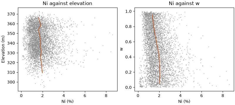
nickel is richer in the lower half of the saprolite. the bedrock moves up and down by tens of meters, so the profile blurs against elevation. against w the decile means explain five times as much of the variance, though most of it stays local.

def binned(x, n=10):
    edges = np.quantile(x, np.linspace(0, 1, n + 1))
    k = np.clip(np.searchsorted(edges, x, side="right") - 1, 0, n - 1)
    means = np.array([ni[k == i].mean() for i in range(n)])
    return (edges[1:] + edges[:-1]) / 2, means, 1 - np.var(ni - means[k]) / np.var(ni)


fig, axes = plt.subplots(1, 2, figsize=(8, 3.6), layout="constrained")
for ax, x, label in zip(axes, [xyz[:, 2], uvw[:, 2]], ["Elevation (m)", "w"], strict=True):
    centers, means, share = binned(x)
    ax.scatter(ni, x, s=2, color=GRAY, linewidths=0)
    ax.plot(means, centers, color=HIGHLIGHT, lw=1.5)
    ax.set(xlabel="Ni (%)", ylabel=label, title=f"Ni against {label.split()[0].lower()}")
    print(f"{label.split()[0]:>9}: decile means explain {share:.1%} of the Ni variance")
save(fig, "profile")

Ni against elevation, Ni against w

Out:

Elevation: decile means explain 1.5% of the Ni variance
        w: decile means explain 7.9% of the Ni variance

variograms¶

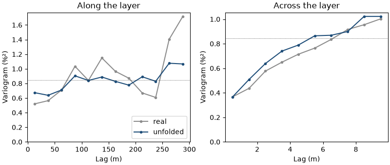
for variography, scale the unfolded w by the mean thickness so that distances across the layer stay in meters. along the layer the pairs are horizontal in the real space and parallel to the surfaces in the unfolded one; across it, they are vertical.

across the layer the two agree at the first lag, and the unfolded variogram rises faster: the holes are vertical, so only the scaling of w changes the distances. along the layer the real variogram starts lower, 0.52 against 0.67 at 12 m: in this deposit nearby samples at one elevation are more alike than nearby samples at one position in the profile.

depth = np.nanmean(thickness)
unfolded = uvw * [1, 1, depth]
spaces = {"real": xyz, "unfolded": unfolded}
fig, axes = plt.subplots(1, 2, figsize=(8, 3.4), layout="constrained")
for (name, coords), color in zip(spaces.items(), [GRAY, ACCENT], strict=True):
    along = bt.experimental_variogram(coords, ni, 25.0, 300.0, azimuth=0, tolerance=90, bandwidth=1.0)
    across = bt.experimental_variogram(coords, ni, 1.0, 10.0, azimuth=0, dip=90, tolerance=10, bandwidth=2.0)
    for ax, e in zip(axes, [along, across], strict=True):
        ax.plot(e.lags, e.gammas, "o-", color=color, ms=3, label=name)
    print(
        f"{name:>8}: gamma along {along.gammas[0]:.2f} at {along.lags[0]:.0f} m, "
        f"across {across.gammas[0]:.2f} at {across.lags[0]:.1f} m"
    )
for ax, title in zip(axes, ["Along the layer", "Across the layer"], strict=True):
    ax.axhline(ni.var(), color=INK, lw=0.6, ls=":")
    ax.set(xlabel="Lag (m)", ylabel="Variogram (%²)", title=title, ylim=(0, None))
axes[0].legend(loc="lower right")
save(fig, "variograms")

Along the layer, Across the layer

Out:

    real: gamma along 0.52 at 12 m, across 0.37 at 0.5 m
unfolded: gamma along 0.67 at 12 m, across 0.37 at 0.5 m

kriging¶

the same ordinary kriging runs on both coordinate sets, cross-validated by leaving out one of ten groups of whole holes at a time.

the variograms predicted it: the real coordinates estimate slightly better, RMSE 0.816 % against 0.865 %. unfolding pays off where grade follows the layer, as in a folded bed or a profile whose base moves more than the grade changes across it. cross-validation on both coordinate sets tells you which case your deposit is.

model = bt.Variogram([("spherical", 0.6 * ni.var(), 150.0)], nugget=0.25 * ni.var(), ratios=(1.0, 0.05))
search = bt.Search(200.0, max_samples=24, ratios=(1.0, 0.05), max_per_hole=6)
kriging = {name: bt.OrdinaryKriging(model, search).fit(c, ni, holes=hole) for name, c in spaces.items()}
for name, k in kriging.items():
    cv = k.cross_validate(folds=10)
    print(f"{name:>8}: RMSE {cv.rmse:.3f} %, correlation {cv.correlation:.3f}")

Out:

    real: RMSE 0.816 %, correlation 0.470
unfolded: RMSE 0.865 %, correlation 0.367

back to the blocks¶

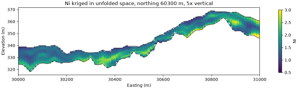
the saprolite blocks are those whose centers unfold to a finite w. their unfolded centers are the kriging targets, and the estimates, one per row, become a column of the real blocks; inverse maps the unfolded centers back onto the centroids. in section the estimates run in bands parallel to the contacts.

blocks = bt.BlockModel(origin=(29975, 59975, 300), size=(10, 10, 1), count=(106, 76, 80))
blocks = blocks.filter(~np.isnan(unfold.transform(blocks)[:, 2]))
targets = unfold.transform(blocks)
back = unfold.inverse(targets)
print(f"inverse of the unfolded centers: {np.abs(back - blocks.coords).max():.1e} m from the centroids")
blocks = blocks.with_column("NI", kriging["unfolded"].predict(targets * [1, 1, depth]))
print(blocks)

north = 60300.0
plane = ((0, north, 0), 90, 90)
fig, ax = plt.subplots(figsize=(10, 3), layout="constrained")
bt.plot.section(blocks, "NI", plane=plane, resolution=1.0, ax=ax, vmin=0.5, vmax=3.0)
bt.plot.slab(np.empty((0, 3)), plane=plane, thickness=10, meshes=[bedrock, limonite], color=INK, ax=ax)
ax.set(title=f"Ni kriged in unfolded space, northing {north:.0f} m, 5x vertical", xlim=(30000, 31000))
ax.set_aspect(5)
save(fig, "section")

Ni kriged in unfolded space, northing 60300 m, 5x vertical

Out:

inverse of the unfolded centers: 0.0e+00 m from the centroids
BlockModel(masked, 87068 of 644480 cells, count [106, 76, 80], size [10.0, 10.0, 1.0], rotation [0.0, 0.0, 0.0])
  NI: Float64

Total running time of the script: ( 0 minutes 0.704 seconds)

Download Python source code: example_04_09.py

Download Jupyter notebook: example_04_09.ipynb

Gallery generated by mkdocs-gallery