locally varying anisotropy¶

walker lake's high-V bodies bend, so one global direction (N170° in variogram fitting) fits some of them and crosses others. locally varying anisotropy (LVA) gives every location its own orientation for both the variogram and the search. the orientation field can come from a gridded attribute (from_grid, used here), a point cloud (from_points) or a wireframe (from_mesh).

import sys
from pathlib import Path

HERE = Path(__file__).parent if "__file__" in globals() else Path.cwd()
sys.path.insert(0, str(HERE.parents[1]))

import boitata as bt
import matplotlib.pyplot as plt
import numpy as np
from common import ACCENT, map_axes, save
from matplotlib.colors import PowerNorm

samples = bt.datasets.walker_lake()
truth = bt.datasets.walker_lake_exhaustive()["V"].reshape(300, 260)
xy, v = samples.coords, samples["V"]
grid = bt.BlockModel(origin=(0.5, 0.5), size=(5, 5), count=(52, 60))
nodes = grid.coords.astype(int)
true_at_nodes = truth[nodes[:, 1] - 1, nodes[:, 0] - 1]

the global model, fitted along N170° and across it as in variogram fitting: two nested structures, with the long one setting the minor/major ratio.

azimuth, lag, max_lag = 170.0, 10.0, 120.0
along = bt.experimental_variogram(xy, v, lag, max_lag, azimuth=azimuth).fit(
    ["spherical", "spherical"], weighting="count/gamma"
)
across = bt.experimental_variogram(xy, v, lag, max_lag, azimuth=azimuth + 90).fit(
    ["spherical", "spherical"],
    weighting="count/gamma",
    nugget=along.nugget,
    sills=[s.sill for s in along.structures],
)
model = along.with_anisotropy(
    (azimuth, 0, 0), (across.structures[-1].range / along.structures[-1].range, 1.0)
)
print(model)

Out:

Variogram(nugget=14993.35122178715, structures=[Structure("spherical", sill=25261.581155025888, range=19.578360959734756), Structure("spherical", sill=53364.6905008533, range=80.65434681410247)], rotation=(170.0, 0.0, 0.0), ratios=(0.33066526059466755, 1.0))

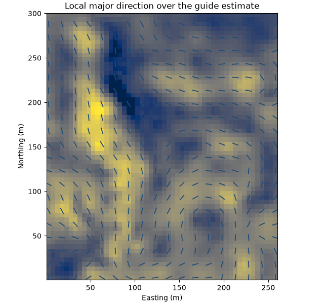
a quick isotropic estimate outlines the bodies, and the gradient of that map gives the orientation of least change. the structure tensor sums gradients over 3 cells each side, and smoothing averages orientations within 25 m.

isotropic = bt.Variogram([("spherical", model.sill - model.nugget, 30.0)], nugget=model.nugget)
guide = bt.OrdinaryKriging(isotropic, bt.Search(radius=60, max_samples=16)).fit(xy, v).predict(grid)
lva = bt.LocalAnisotropy.from_grid(
    grid.with_column("guide", guide), "guide", window=3, ratios=(0.3, 1.0)
).smooth(25.0)
print(lva)
print("azimuth percentiles (10, 50, 90):", np.percentile(lva.angles[:, 0] % 180, [10, 50, 90]).round())

Out:

LocalAnisotropy(3120 locations)
azimuth percentiles (10, 50, 90): [ 17. 113. 172.]

extent = (0.5, 260.5, 0.5, 300.5)
fig, ax = plt.subplots(figsize=(6.4, 6), layout="constrained")
ax.imshow(
    grid.grid(guide)[0],
    origin="lower",
    extent=extent,
    cmap="cividis",
    norm=PowerNorm(0.5, vmin=0, vmax=1200),
)
every = (nodes[:, 0] % 15 == 3) & (nodes[:, 1] % 15 == 3)
bt.plot.directions(lva.at(grid.coords[every]), ax=ax, scale=35, width=0.004, color=ACCENT)
map_axes(ax, "Local major direction over the guide estimate")
save(fig, "field")

Local major direction over the guide estimate

same model, same search; only the orientation changes. errors are against the exhaustive values at the nodes.

search = bt.Search(radius=100, max_samples=24, min_samples=4)
ok = bt.OrdinaryKriging(model, search).fit(xy, v)
global_estimate = ok.predict(grid)
local_estimate = ok.predict(grid, anisotropy=lva)
for name, estimate in ((f"global N{model.rotation[0]:.0f}°", global_estimate), ("local", local_estimate)):
    score = bt.compare(estimate, true_at_nodes)
    print(f"{name:>13}: RMSE {score['rmse']:.1f} ppm, correlation {score['correlation']:.3f}")

Out:

 global N170°: RMSE 157.3 ppm, correlation 0.780
        local: RMSE 148.3 ppm, correlation 0.805

norm = PowerNorm(0.5, vmin=0, vmax=1500)
fig, axes = plt.subplots(1, 3, figsize=(12, 4.6), layout="constrained")
for ax, image, title in (
    (axes[0], true_at_nodes, "True V at grid nodes"),
    (axes[1], global_estimate, "Kriging, global anisotropy"),
    (axes[2], local_estimate, "Kriging, local anisotropy"),
):
    im = ax.imshow(grid.grid(image)[0], origin="lower", extent=extent, norm=norm)
    map_axes(ax, title)
fig.colorbar(im, ax=axes, shrink=0.8, label="V (ppm)")
save(fig, "kriging")

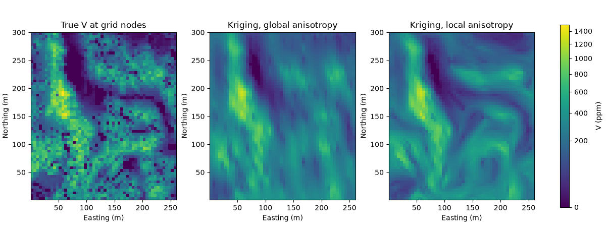
True V at grid nodes, Kriging, global anisotropy, Kriging, local anisotropy

local orientations lower the error and keep the north-eastern bodies elongated east-west, where the global direction crosses them.

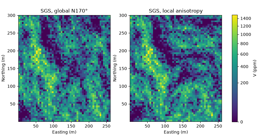
simulation takes the same field: each node's variogram and search follow the local direction, so continuity bends with the bodies instead of crossing them. the normal-score variogram is fitted along the major axis; the field supplies the orientation and the ratios.

weights = bt.cell_declustering(xy, v, sizes=np.arange(2.5, 102.5, 2.5)).weights
scores = bt.NormalScore().fit_transform(v, weights=weights)
gaussian = bt.experimental_variogram(xy, scores, lag, max_lag, azimuth=azimuth).fit("spherical")
sgs = bt.SGS(gaussian, bt.Search(radius=100, max_samples=24)).fit(xy, v, weights=weights)
uniform = bt.LocalAnisotropy(np.zeros((1, 3)), [model.rotation], [model.ratios])
global_real = sgs.simulate(grid, n=1, seed=11, keep=True, anisotropy=uniform).realizations[0]
local_real = sgs.simulate(grid, n=1, seed=11, keep=True, anisotropy=lva).realizations[0]

fig, axes = plt.subplots(1, 2, figsize=(8.6, 4.6), layout="constrained")
for ax, image, title in (
    (axes[0], global_real, f"SGS, global N{model.rotation[0]:.0f}°"),
    (axes[1], local_real, "SGS, local anisotropy"),
):
    im = ax.imshow(grid.grid(image)[0], origin="lower", extent=extent, norm=norm)
    map_axes(ax, title)
fig.colorbar(im, ax=axes, shrink=0.8, label="V (ppm)")
save(fig, "simulation")