discrete gaussian model¶

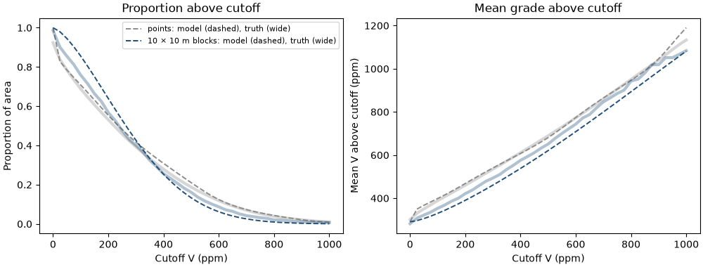
mining selects blocks. block grades vary less than point grades, so a point histogram misstates the tonnage above cutoffs. the discrete gaussian model shrinks a hermite anamorphosis of the points to block support, and the exhaustive walker lake grid gives the true point and block curves to check it against.

import sys
from pathlib import Path

HERE = Path(__file__).parent if "__file__" in globals() else Path.cwd()
sys.path.insert(0, str(HERE.parents[1]))

import boitata as bt
import matplotlib.pyplot as plt
import numpy as np
from common import ACCENT, GRAY, save

samples = bt.datasets.walker_lake()
truth = bt.datasets.walker_lake_exhaustive()["V"].reshape(300, 260)
xy, v = samples.coords, samples["V"]
weights = bt.cell_declustering(samples, "V", sizes=np.arange(2.5, 102.5, 2.5)).weights

a hermite anamorphosis models the declustered point distribution. the variogram of its gaussian scores is fitted jointly along and across N170°, the major axis found in variogram fitting:

anam = bt.HermiteAnamorphosis(degree=40).fit(v, weights=weights)
y = anam.transform(v)
azimuths = (170, 260)
experimental = [bt.experimental_variogram(xy, y, 10, 120, azimuth=a) for a in azimuths]
gaussian = bt.Variogram.fit_directional(experimental, [(a, 0) for a in azimuths], rotation=[170, 0, 0])
print(gaussian)

Out:

Variogram(nugget=0.3880895785084983, structures=[Structure("spherical", sill=0.6541303654567798, range=95.35466468171232)], rotation=(170.0, 0.0, 0.0), ratios=(0.3490856295281619, 1.0))

change_of_support averages the gaussian correlogram over a 10 × 10 m block and returns the change-of-support coefficient r with the block anamorphosis. only the correlogram matters, so the sill of the variogram has no effect.

size = 10
r, block = bt.change_of_support(anam, gaussian, size=(size, size), discretization=(5, 5, 1))
blocks_true = truth.reshape(30, size, 26, size).mean(axis=(1, 3)).ravel()
print(
    f"r = {r:.3f}; point variance {anam.variance_:.0f}, block {block.variance_:.0f}, true block {blocks_true.var():.0f}"
)

Out:

r = 0.725; point variance 64974, block 32652, true block 46694

grade-tonnage curves, model against truth:

cutoffs = np.linspace(0, 1000, 41)
model_point = anam.grade_tonnage(cutoffs)
model_block = block.grade_tonnage(cutoffs)


def empirical(values):
    tonnage = np.array([(values > c).mean() for c in cutoffs])
    grade = np.array([values[values > c].mean() if (values > c).any() else np.nan for c in cutoffs])
    return tonnage, grade


true_point = empirical(truth.ravel())
true_block = empirical(blocks_true)
for c in (300, 500, 800):
    k = np.searchsorted(cutoffs, c)
    print(
        f"above {c} ppm: points {model_point['tonnage'][k]:.1%} (true {true_point[0][k]:.1%}), "
        f"blocks {model_block['tonnage'][k]:.1%} (true {true_block[0][k]:.1%})"
    )

fig, (a, b) = plt.subplots(1, 2, figsize=(10, 3.8), layout="constrained")
for curves, model, color, label in (
    (true_point, model_point, GRAY, "points"),
    (true_block, model_block, ACCENT, f"{size} × {size} m blocks"),
):
    a.plot(cutoffs, curves[0], color=color, lw=3, alpha=0.35)
    a.plot(
        cutoffs,
        model["tonnage"],
        color=color,
        lw=1.4,
        ls="--",
        label=f"{label}: model (dashed), truth (wide)",
    )
    b.plot(cutoffs, curves[1], color=color, lw=3, alpha=0.35)
    b.plot(cutoffs, model["mean_grade"], color=color, lw=1.4, ls="--")
a.set(title="Proportion above cutoff", xlabel="Cutoff V (ppm)", ylabel="Proportion of area")
a.legend(fontsize=8)
b.set(title="Mean grade above cutoff", xlabel="Cutoff V (ppm)", ylabel="Mean V above cutoff (ppm)")
save(fig, "grade-tonnage")

Proportion above cutoff, Mean grade above cutoff

Out:

above 300 ppm: points 41.7% (true 39.3%), blocks 42.7% (true 40.1%)
above 500 ppm: points 21.1% (true 18.8%), blocks 13.3% (true 16.2%)
above 800 ppm: points 4.3% (true 3.9%), blocks 1.0% (true 2.1%)

the model shrinks the point variance of 64 974 to 32 652 for 10 m blocks, below the true 46 694, so it pulls the rich tail in too far: above 500 ppm it keeps 13.3% of the blocks against a true 16.2%, above 800 ppm 1.0% against 2.1%. the point curves run a few percent high, since the declustered samples still overstate the rich grades. uniform conditioning and MIK localization carry block support down to panels; simulation at block support reaches it by simulation.

Total running time of the script: ( 0 minutes 0.226 seconds)

Download Python source code: example_09_01.py

Download Jupyter notebook: example_09_01.ipynb

Gallery generated by mkdocs-gallery