Note
Click here to download the full example code
Grade-tonnage curves and the change in contained metal
Compare two estimates chose the ordinary kriging over the inverse distance model of Walker Lake. Management asks the next question: how much metal does that decision remove from the resource? You build grade-tonnage curves for both models and for the true blocks, report tonnes, grade and metal at a set of cutoffs, state the change in contained metal at the reporting cutoff, and check that the metal adds up.
import sys
from pathlib import Path

HERE = Path(__file__).parent if "__file__" in globals() else Path.cwd()
sys.path.insert(0, str(HERE.parents[1]))
import boitata as bt
import matplotlib.pyplot as plt
import numpy as np
from common import ACCENT, HIGHLIGHT, INK, save
What you'll learn
- What a grade-tonnage curve reports: tonnes, mean grade and metal above each cutoff.
- Why a smooth estimate reports more tonnes at a lower grade above a low cutoff.
- How to state a change in contained metal in absolute and relative terms, and check that it balances.
Prerequisites: compare two estimates, which builds the two models.
Result plots documents bt.plot.grade_tonnage.
The data
The blocks are those of the previous tutorial: 26 × 30 blocks of 10 × 10 m. A grade-tonnage report needs tonnes,
which Walker Lake does not have, so two assumptions give them: a 10 m bench centered on the sample plane, and a
density of 2.7 t/m³. Each block is then 10 × 10 × 10 m = 1 000 m³ and weighs 2 700 t. Walker Lake's V is read
as a grade in ppm (g/t), so tonnes × ppm gives grams of metal; the tables below divide by 10⁶ to report tonnes of
metal.
samples = bt.datasets.walker_lake()
xy, v = samples.coords, samples["V"]
azimuths = np.arange(0, 180, 22.5)
directional = [bt.experimental_variogram(xy, v, 10.0, 120.0, azimuth=a) for a in azimuths]
model = bt.Variogram.fit_directional(
    directional, [(a, 0) for a in azimuths], ["spherical", "spherical"], weighting="count/gamma"
)
search = bt.Search(radius=80, max_samples=24, min_samples=4, rotation=model.rotation, ratios=(0.5, 1.0))
kriging = bt.BlockKriging(model, search, size=(10, 10), discretization=(5, 5, 1)).fit(xy, v)
inverse = bt.InverseDistance(search, power=2).fit(xy, v)

density = 2.7
blocks = bt.BlockModel(origin=(0.5, 0.5, -5.0), size=(10, 10, 10), count=(26, 30, 1))
truth = bt.datasets.walker_lake_exhaustive()["V"].reshape(300, 260)
blocks = blocks.with_columns(
    {
        "ok": kriging.predict(blocks),
        "id": inverse.predict(blocks),
        "truth": truth.reshape(30, 10, 26, 10).mean(axis=(1, 3)).ravel(),
    }
)
tonnes = 10 * 10 * 10 * density
print(blocks)
print(f"{blocks['ok'].size} blocks × {tonnes:,.0f} t = {blocks['ok'].size * tonnes:,.0f} t")
Out:
BlockModel(regular, 780 of 780 cells, count [26, 30, 1], size [10.0, 10.0, 10.0], rotation [0.0, 0.0, 0.0])
  ok: Float64
  id: Float64
  truth: Float64
780 blocks × 2,700 t = 2,106,000 t
The true blocks are the averages of the exhaustive grid over each block. A real deposit has no such column; here it shows which model reports the right tonnes.
Step 1: One grade-tonnage curve
For a cutoff \(c\), the tonnage is the sum of the tonnes of the blocks with grade ≥ \(c\), the mean grade is
their tonne-weighted average, and the metal is tonnage × mean grade. grade_tonnage computes this for a list
of cutoffs. data=blocks lets it read the column by name and use each block's volume as its weight;
density turns volume into tonnes.
cutoffs = np.arange(0, 1001, 25.0)
curve = bt.grade_tonnage("ok", cutoffs, density=density, data=blocks)
print(curve.column_names)
for row in zip(*(curve[c] for c in ("cutoff", "tonnage", "mean_grade", "metal"))):
    if row[0] in (0, 200, 400):
        cutoff, t, g, m = row
        print(f"cutoff {cutoff:3.0f} ppm: {t / 1e6:.3f} Mt at {g:.1f} ppm = {m / 1e6:.1f} t of metal")
Out:
['cutoff', 'tonnage', 'mean_grade', 'metal']
cutoff   0 ppm: 2.106 Mt at 291.7 ppm = 614.2 t of metal
cutoff 200 ppm: 1.353 Mt at 388.3 ppm = 525.2 t of metal
cutoff 400 ppm: 0.464 Mt at 568.8 ppm = 264.1 t of metal
The math
With block tonnes \(t_i\) and grades \(z_i\), for a cutoff \(c\): [ T(c) = \sum_{z_i \ge c} t_i, \qquad M(c) = \sum_{z_i \ge c} t_i z_i, \qquad \bar z(c) = M(c) / T(c). ] At \(c = 0\) the metal is the whole model's, \(\sum_i t_i z_i\).
Step 2: All three models on one set of cutoffs
compare_models repeats grade_tonnage for several columns of one block model (a dict names each one) and
adds each model's difference from a reference. The true blocks are the reference here, to see which model
is closer.
labels = {"truth": "true blocks", "ok": "kriging", "id": "inverse distance"}
columns = {label: name for name, label in labels.items()}
table = bt.compare_models(blocks, columns, cutoffs, reference="true blocks", density=density)


def at(table, name, cutoff):
    rows = (table["model"] == labels[name]) & (table["cutoff"] == cutoff)
    return {
        c: float(table[c][rows][0])
        for c in ("tonnage", "mean_grade", "metal", "tonnage_diff", "grade_diff", "metal_diff")
    }


print(
    f"{'cutoff':>6} {'model':>16} {'kt':>7} {'V ppm':>6} {'metal t':>8}   vs truth: {'t':>6} {'grade':>6} {'metal':>6}"
)
for cutoff in (0, 100, 200, 300, 400, 600):
    for name, label in labels.items():
        r = at(table, name, cutoff)
        print(
            f"{cutoff:6.0f} {label:>16} {r['tonnage'] / 1e3:7.1f} {r['mean_grade']:6.1f} {r['metal'] / 1e6:8.1f}"
            f"             {r['tonnage_diff']:+6.1%} {r['grade_diff']:+6.1%} {r['metal_diff']:+6.1%}"
        )
Out:
cutoff            model      kt  V ppm  metal t   vs truth:      t  grade  metal
     0      true blocks  2106.0  278.0    585.4              +0.0%  +0.0%  +0.0%
     0          kriging  2106.0  291.7    614.2              +0.0%  +4.9%  +4.9%
     0 inverse distance  2106.0  332.8    700.8              +0.0% +19.7% +19.7%
   100      true blocks  1598.4  353.3    564.7              +0.0%  +0.0%  +0.0%
   100          kriging  1833.3  326.1    597.9             +14.7%  -7.7%  +5.9%
   100 inverse distance  1930.5  356.9    688.9             +20.8%  +1.0% +22.0%
   200      true blocks  1196.1  421.3    504.0              +0.0%  +0.0%  +0.0%
   200          kriging  1352.7  388.3    525.2             +13.1%  -7.8%  +4.2%
   200 inverse distance  1571.4  403.1    633.4             +31.4%  -4.3% +25.7%
   300      true blocks   845.1  493.6    417.1              +0.0%  +0.0%  +0.0%
   300          kriging   882.9  462.0    407.9              +4.5%  -6.4%  -2.2%
   300 inverse distance  1150.2  458.6    527.4             +36.1%  -7.1% +26.4%
   400      true blocks   540.0  575.8    310.9              +0.0%  +0.0%  +0.0%
   400          kriging   464.4  568.8    264.1             -14.0%  -1.2% -15.0%
   400 inverse distance   683.1  533.9    364.7             +26.5%  -7.3% +17.3%
   600      true blocks   183.6  743.5    136.5              +0.0%  +0.0%  +0.0%
   600          kriging   137.7  762.4    105.0             -25.0%  +2.5% -23.1%
   600 inverse distance   162.0  729.0    118.1             -11.8%  -2.0% -13.5%
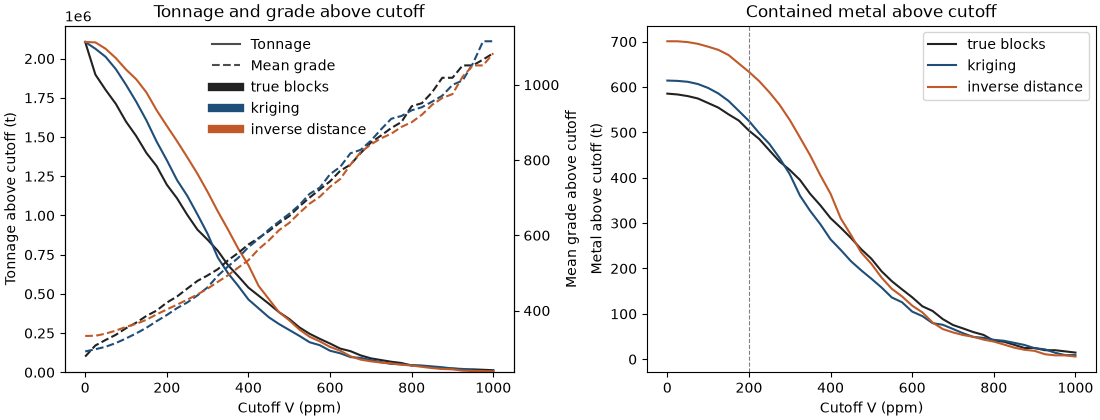
Read the kriging rows against the truth. At 100 and 200 ppm kriging reports 14.7 % and 13.1 % too many tonnes at a grade 7.7 % and 7.8 % too low; the metal is off by 5.9 % and 4.2 %, because the two errors partly cancel. From 400 ppm up kriging reports too few tonnes (−14.0 % at 400, −25.0 % at 600). Figure 1 shows why.
Key idea
Estimation averages neighboring samples, so estimated blocks vary less than true blocks. Above a low cutoff, a smooth model lifts waste blocks over the cutoff, adding tonnes and diluting the grade. Above a high cutoff, it pulls the rich blocks down under it and loses tonnes. Tonnage and grade move in opposite directions at low cutoffs, so the error in metal is smaller than the error in tonnes.
Step 3: Draw the curves
bt.plot.grade_tonnage draws the compare_models table: tonnage solid on the left axis, mean grade
dashed on the right, one color per model. Metal above cutoff is a third curve worth its own panel.
fig, (a, b) = plt.subplots(1, 2, figsize=(11, 4.2), layout="constrained")
with plt.rc_context({"axes.prop_cycle": plt.cycler(color=[INK, ACCENT, HIGHLIGHT])}):
    bt.plot.grade_tonnage(table, ax=a)
a.set(xlabel="Cutoff V (ppm)", ylabel="Tonnage above cutoff (t)", title="Tonnage and grade above cutoff")
for name, color in (("truth", INK), ("ok", ACCENT), ("id", HIGHLIGHT)):
    rows = table["model"] == labels[name]
    b.plot(cutoffs, table["metal"][rows] / 1e6, color=color, label=labels[name])
b.axvline(200, color="gray", lw=0.8, ls="--")
b.set(xlabel="Cutoff V (ppm)", ylabel="Metal above cutoff (t)", title="Contained metal above cutoff")
b.legend()
save(fig, "grade_tonnage")
Step 4: The change in contained metal at the reporting cutoff
The resource is reported above 200 ppm (the dashed line). Replacing the inverse distance model by the kriging changes the reported numbers as follows.
report = 200
old, new, true = (at(table, name, report) for name in ("id", "ok", "truth"))
for key, unit, scale in (("tonnage", "kt", 1e3), ("mean_grade", "ppm", 1), ("metal", "t", 1e6)):
    change = new[key] - old[key]
    print(
        f"{key:>10}: inverse distance {old[key] / scale:8.1f}, kriging {new[key] / scale:8.1f} {unit:>3}, "
        f"change {change / scale:+8.1f} {unit} ({change / old[key]:+.1%}); truth {true[key] / scale:8.1f}"
    )
Out:
   tonnage: inverse distance   1571.4, kriging   1352.7  kt, change   -218.7 kt (-13.9%); truth   1196.1
mean_grade: inverse distance    403.1, kriging    388.3 ppm, change    -14.8 ppm (-3.7%); truth    421.3
     metal: inverse distance    633.4, kriging    525.2   t, change   -108.2 t (-17.1%); truth    504.0
Switching to kriging removes 218.7 kt (−13.9 %), 14.8 ppm of grade (−3.7 %) and 108.2 t of metal (−17.1 %). Kriging's 525.2 t is still 4.2 % above the true 504.0 t; inverse distance was 25.7 % above it. At cutoff 0, where no block is selected out, inverse distance holds 19.7 % more metal than the truth, against 4.9 % for kriging: most of its excess is the clustering bias of the previous tutorial.
Pitfall: quoting only the tonnage change
"Kriging loses 13.9 % of the tonnes" is not the metal change, which is 17.1 % here. Tonnage alone can get the sign wrong: at 300 ppm kriging reports 4.5 % more tonnes than the truth but 2.2 % less metal. Report tonnes, grade and metal together, each in absolute and relative terms.
Check before you move on
Metal must balance three ways: the reported metal equals tonnage × mean grade at every cutoff; at cutoff 0 it equals block tonnes × grade summed over all blocks; and above the reporting cutoff it equals the same sum over the blocks at or above the cutoff.
for name, label in labels.items():
    rows = table["model"] == label
    t, g, m = (table[c][rows] for c in ("tonnage", "mean_grade", "metal"))
    above = ~np.isnan(g)
    assert np.allclose(m[above], t[above] * g[above])
    grade = blocks[name]
    total = (tonnes * grade).sum()
    selected = (tonnes * grade[grade >= report]).sum()
    assert np.isclose(m[0], total) and np.isclose(at(table, name, report)["metal"], selected)
    print(
        f"{label:>16}: metal at cutoff 0 {m[0] / 1e6:5.1f} t = sum over blocks {total / 1e6:5.1f} t; "
        f"above {report} ppm {selected / 1e6:5.1f} t in {(grade >= report).sum()} blocks"
    )
Out:
     true blocks: metal at cutoff 0 585.4 t = sum over blocks 585.4 t; above 200 ppm 504.0 t in 443 blocks
         kriging: metal at cutoff 0 614.2 t = sum over blocks 614.2 t; above 200 ppm 525.2 t in 501 blocks
inverse distance: metal at cutoff 0 700.8 t = sum over blocks 700.8 t; above 200 ppm 633.4 t in 582 blocks
All three models balance: for kriging, 614.2 t in the whole model, 525.2 t of it in the 501 blocks above 200 ppm. A metal figure that does not balance usually means blocks without a grade (null) were counted in the tonnes, or the density was applied twice.
The decision
Report the kriging: 1 352.7 kt at 388.3 ppm, 525.2 t of metal above 200 ppm. The change from the scoping model is −108.2 t of metal (−17.1 %), which the clustering bias found in compare two estimates explains. The remaining smoothing (too many tonnes at too low a grade at this cutoff) is a change-of-support problem: the discrete Gaussian model and uniform conditioning estimate the tonnage a selective mining unit would recover.
Total running time of the script: ( 0 minutes 0.342 seconds)
Download Python source code: example_14_06.py