simple estimators¶

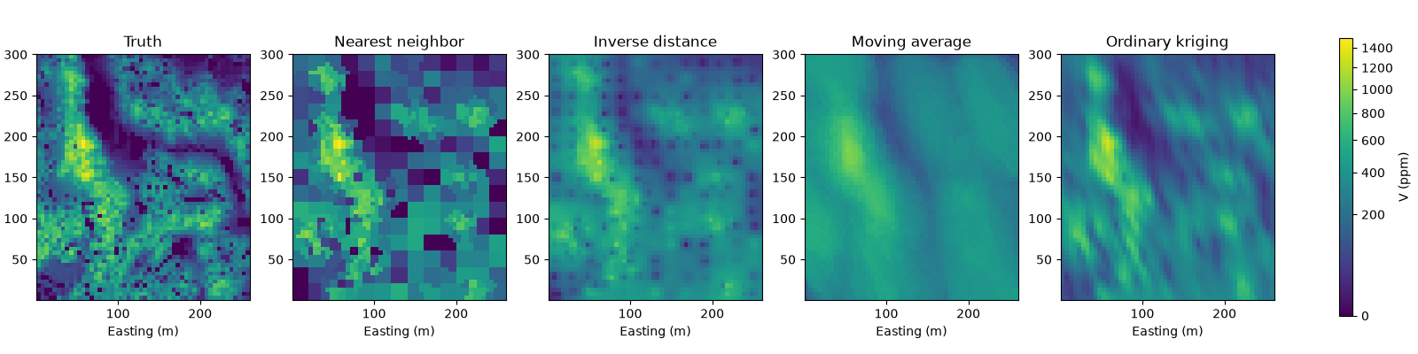
nearest neighbor, inverse distance and moving average estimate walker lake V without a variogram. they use the same 470 samples and neighborhood as ordinary kriging and are checked against the exhaustive values; compare_models sets their grade-tonnage curves against the truth.

import sys
from pathlib import Path

HERE = Path(__file__).parent if "__file__" in globals() else Path.cwd()
sys.path.insert(0, str(HERE.parents[1]))

import boitata as bt
import matplotlib.pyplot as plt
import numpy as np
from common import ACCENT, GRAY, HIGHLIGHT, INK, map_axes, save
from matplotlib.colors import PowerNorm

samples = bt.datasets.walker_lake()
truth = bt.datasets.walker_lake_exhaustive()["V"].reshape(300, 260)
grid = bt.BlockModel(origin=(0.5, 0.5), size=(5, 5), count=(52, 60))
nodes = grid.coords.astype(int)
true_at_nodes = truth[nodes[:, 1] - 1, nodes[:, 0] - 1]

azimuths = np.arange(0, 180, 22.5)
directional = [bt.experimental_variogram(samples, "V", 10.0, 120.0, azimuth=a) for a in azimuths]
model = bt.Variogram.fit_directional(
    directional, [(a, 0) for a in azimuths], ["spherical", "spherical"], weighting="count/gamma"
)

all four share one search: up to 24 samples in an ellipse along the direction of greatest continuity. nearest neighbor takes the closest sample, inverse distance weights by 1/d², and moving average weights all neighbors equally. kriging, the reference, uses the variogram above.

search = bt.Search(radius=80, max_samples=24, min_samples=4, rotation=model.rotation, ratios=(0.5, 1.0))
methods = {
    "nearest neighbor": bt.NearestNeighbor(search),
    "inverse distance": bt.InverseDistance(search, power=2),
    "moving average": bt.MovingAverage(search),
    "ordinary kriging": bt.OrdinaryKriging(model, search),
}
estimates = {name: m.fit(samples, "V").predict(grid) for name, m in methods.items()}
print(f"{'method':>17}  RMSE   corr   variance ratio")
for name, e in estimates.items():
    ok = ~np.isnan(e)
    score = bt.compare(e, true_at_nodes)
    print(
        f"{name:>17}  {score['rmse']:5.1f}  {score['correlation']:.3f}  {e[ok].var() / true_at_nodes[ok].var():.2f}"
    )

Out:

           method  RMSE   corr   variance ratio
 nearest neighbor  178.5  0.739  0.95
 inverse distance  166.2  0.777  0.55
   moving average  231.0  0.586  0.30
 ordinary kriging  155.1  0.786  0.62

nearest neighbor keeps almost all the variance but places it poorly, as a patchwork of polygons around the samples. moving average smooths the most and is the least accurate, since distant samples weigh as much as close ones. inverse distance sits between them and comes close to kriging, the most accurate here. kriging also gives a variance per estimate and accounts for clustered samples, which inverse distance does not.

extent = (0.5, 260.5, 0.5, 300.5)
norm = PowerNorm(0.5, vmin=0, vmax=1500)
fig, axes = plt.subplots(1, 5, figsize=(16, 4), layout="constrained")
for ax, (title, image) in zip(axes, [("truth", true_at_nodes), *estimates.items()]):
    im = ax.imshow(grid.grid(image)[0], origin="lower", extent=extent, norm=norm)
    map_axes(ax, title.capitalize())
    ax.set_ylabel("")
fig.colorbar(im, ax=axes, shrink=0.8, label="V (ppm)")
save(fig, "methods")

Truth, Nearest neighbor, Inverse distance, Moving average, Ordinary kriging

grade-tonnage¶

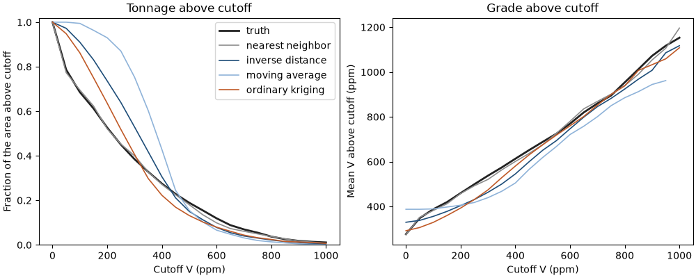
smoothing shows in selection. for each cutoff, compare_models computes the tonnage, mean grade and metal above it for every model of the same blocks, and their differences from a reference, here the truth at the nodes.

cutoffs = np.arange(0, 1001, 50)
table = bt.compare_models(grid, {"truth": true_at_nodes, **estimates}, cutoffs, reference="truth")
for cutoff in (300, 600):
    rows = table["cutoff"] == cutoff
    print(f"cutoff {cutoff} ppm")
    for name, t, g in zip(table["model"][rows], table["tonnage_diff"][rows], table["grade_diff"][rows]):
        print(f"  {name:>17}: tonnage {t:+.0%}, grade {g:+.0%}")

colors = [INK, GRAY, ACCENT, "#8fb3d9", HIGHLIGHT]
fig, (a, b) = plt.subplots(1, 2, figsize=(10, 4), layout="constrained")
for name, color in zip(["truth", *estimates], colors):
    rows = table["model"] == name
    tonnage = table["tonnage"][rows]
    a.plot(cutoffs, tonnage / tonnage[0], color=color, lw=2 if name == "truth" else 1.2, label=name)
    b.plot(cutoffs, table["mean_grade"][rows], color=color, lw=2 if name == "truth" else 1.2)
a.set(xlabel="Cutoff V (ppm)", ylabel="Fraction of the area above cutoff", ylim=(0, 1.02))
a.set_title("Tonnage above cutoff")
a.legend()
b.set(xlabel="Cutoff V (ppm)", ylabel="Mean V above cutoff (ppm)")
b.set_title("Grade above cutoff")
save(fig, "grade_tonnage")

Tonnage above cutoff, Grade above cutoff

Out:

cutoff 300 ppm
              truth: tonnage +0%, grade +0%
   nearest neighbor: tonnage +4%, grade -3%
   inverse distance: tonnage +38%, grade -14%
     moving average: tonnage +96%, grade -18%
   ordinary kriging: tonnage +6%, grade -12%
cutoff 600 ppm
              truth: tonnage +0%, grade +0%
   nearest neighbor: tonnage -17%, grade +1%
   inverse distance: tonnage -34%, grade -3%
     moving average: tonnage -45%, grade -6%
   ordinary kriging: tonnage -33%, grade -1%

smooth estimates put too much of the area above a low cutoff and too little above a high one: at 300 ppm moving average nearly doubles the true tonnage, and at 600 ppm it misses 45 % of it. nearest neighbor follows the true tonnage because it keeps the variance of the data, yet its local estimates are wrong. a reliable grade-tonnage of selected blocks needs a change of support (the discrete gaussian model and the pages after it).

Total running time of the script: ( 0 minutes 0.621 seconds)

Download Python source code: example_06_02.py

Download Jupyter notebook: example_06_02.ipynb

Gallery generated by mkdocs-gallery