Note

Click here to download the full example code

SGS along a shared path

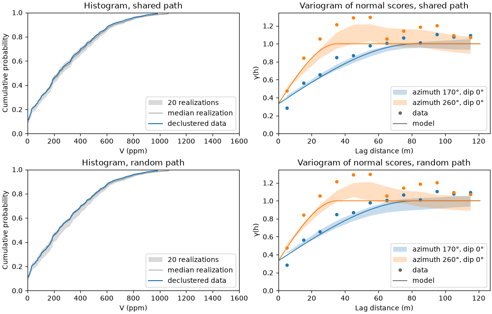
on a block model, SGS runs all realizations along one multigrid path: coarse cells first, then finer ones. a node's neighbors and kriging weights then depend on the path alone, so SGS finds them once per batch of realizations and reuses them; only the noise differs. path="random" draws a new path per realization instead, as points and sub-blocked models need. both reproduce the histogram and the variogram, and the shared path gains speed as realizations and nodes grow. batch, the number simulated together, leaves the realizations unchanged and by default fills 70 % of the free memory.

import sys
import time
from pathlib import Path

HERE = Path(__file__).parent if "__file__" in globals() else Path.cwd()
sys.path.insert(0, str(HERE.parents[1]))

import boitata as bt
import matplotlib.pyplot as plt
import numpy as np
from common import save

walker lake V, simulated as in realization checks on a 1 m grid of 260 × 300 cells: declustered normal scores and their variogram along N170° and across it.

samples = bt.datasets.walker_lake()
xy, v = samples.coords, samples["V"]
weights = bt.cell_declustering(xy, v, sizes=np.arange(2.5, 102.5, 2.5)).weights
y = bt.NormalScore(tails=(0.0, v.max())).fit_transform(v, weights=weights)

azimuth, lag, max_lag = 170.0, 10.0, 120.0
major = bt.experimental_variogram(xy, y, lag, max_lag, azimuth=azimuth).fit("spherical")
minor = bt.experimental_variogram(xy, y, lag, max_lag, azimuth=azimuth + 90).fit("spherical")
ratio = min(minor.structures[0].range / major.structures[0].range, 1.0)
gaussian = major.standardized().with_anisotropy((azimuth, 0, 0), (ratio, 1.0))
grid = bt.BlockModel(origin=(0.5, 0.5), size=(1, 1), count=(260, 300))
sgs = bt.SGS(gaussian, bt.Search(radius=100, max_samples=24)).fit(samples, "V", weights=weights)

twenty realizations along each kind of path, timed:

runs = {}
for path in ["shared", "random"]:
    start = time.perf_counter()
    runs[path] = sgs.simulate(grid, n=20, seed=42, keep=True, path=path)
    print(
        f"{path:6} path: {time.perf_counter() - start:5.2f} s for 20 realizations of {len(grid.coords):,} nodes"
    )

Out:

shared path:  0.24 s for 20 realizations of 78,000 nodes
random path:  1.87 s for 20 realizations of 78,000 nodes

batch changes memory and speed and leaves the realizations alone: one at a time gives the same grades as all together.

one = sgs.simulate(grid, n=4, seed=42, keep=True, path="shared", batch=1)
together = sgs.simulate(grid, n=4, seed=42, keep=True, path="shared", batch=4)
print("batch=1 equals batch=4:", np.array_equal(one.realizations, together.realizations))

Out:

batch=1 equals batch=4: True

both paths reproduce the declustered histogram and the variogram model along N170°; the bands overlap.

fig, axes = plt.subplots(2, 2, figsize=(10, 6.4), layout="constrained")
for row, (path, summary) in zip(axes, runs.items()):
    check = bt.check_realizations(
        grid, summary, samples, "V", weights=weights, variogram=gaussian, lag=lag, max_lag=max_lag
    )
    bt.plot.histogram_reproduction(check, ax=row[0])
    bt.plot.variogram_reproduction(check, ax=row[1])
    row[0].set(xlim=(0, 1600), xlabel="V (ppm)", title=f"Histogram, {path} path")
    row[1].set(xlabel="Lag distance (m)", title=f"Variogram of normal scores, {path} path")
save(fig, "reproduction")

Total running time of the script: ( 0 minutes 19.937 seconds)

Download Python source code: example_08_02.py

Download Jupyter notebook: example_08_02.ipynb

Gallery generated by mkdocs-gallery