grades in simulated rock types¶

a grade simulated within a fixed rock-type model ignores the uncertainty of the contacts. given one rock-type realization per grade realization, SGS simulates realization k of the grade within realization k of the rock types, so the grade maps carry that uncertainty too.

import sys
from pathlib import Path

HERE = Path(__file__).parent if "__file__" in globals() else Path.cwd()
sys.path.insert(0, str(HERE.parents[1]))

import boitata as bt
import matplotlib.pyplot as plt
import numpy as np
from common import save

rock types¶

jura's rock types are known at each node of the prediction grid. SIS (sequential indicator simulation) draws 10 rock-type realizations from indicator variograms fitted to the samples; portlandian, with 3 samples, gets a guessed one.

jura = bt.datasets.jura()
train, grid = jura["prediction"], jura["grid"]
names = ["Argovian", "Kimmeridgian", "Sequanian", "Portlandian", "Quaternary"]
rock_types = bt.Categories(names)
rock = rock_types.encode(train["Rock"]).astype(int)
true_rock = rock_types.encode(grid["Rock"]).astype(int)

indicator_variograms = []
for k in range(5):
    indicator = (rock == k).astype(float)
    if indicator.sum() >= 5:
        fitted = bt.experimental_variogram(train.coords, indicator, 0.1, 1.5).fit("spherical")
    else:
        fitted = bt.Variogram([("spherical", indicator.var(), 0.5)])
    indicator_variograms.append(fitted)
sis = bt.SIS(indicator_variograms, bt.Search(radius=1.5, max_samples=16)).fit(train, rock)
by_sis = sis.simulate(grid, n=10, seed=3, keep=True).realizations
print(f"rock-type realizations: {by_sis.shape}")
print(f"{'Co (ppm)':<14}{'samples':>8}{'mean':>7}")
for k, name in enumerate(names):
    print(f"{name:<14}{np.sum(rock == k):8d}{train['Co'][rock == k].mean():7.2f}")

Out:

rock-type realizations: (10, 5957)
Co (ppm)       samples   mean
Argovian            53   5.39
Kimmeridgian        85  11.05
Sequanian           63   9.98
Portlandian          3   9.37
Quaternary          55   9.60

grades within the rock types¶

fitted with domains, SGS normal-scores Co within each rock type, so the lean argovian keeps its own distribution. the variogram here fits scores computed per rock type the same way. at simulate, domains takes one of two forms. one row of labels (here the true rock types) holds the domains fixed; an array of shape (n, targets) (here the SIS realizations) gives each Co realization its own rock-type map.

co = train["Co"]
co_scores = np.empty(len(co))
for k in range(5):
    co_scores[rock == k] = bt.NormalScore().fit_transform(co[rock == k])
co_variogram = bt.experimental_variogram(train.coords, co_scores, 0.1, 1.5).fit("spherical")
cobalt = bt.SGS(co_variogram, bt.Search(radius=1.5, max_samples=16)).fit(train, "Co", domains=rock)
within_true = cobalt.simulate(grid, n=10, seed=3, keep=True, domains=true_rock).realizations
within_sis = cobalt.simulate(grid, n=10, seed=3, keep=True, domains=by_sis).realizations

argovian = (by_sis == 0).mean(axis=0)
unsure = (argovian > 0) & (argovian < 1)
print(f"{'Co (ppm)':<42}{'true rock types':>16}{'SIS rock types':>16}")
rows = [
    ("mean", lambda r: r.mean()),
    ("mean on true Argovian", lambda r: r[:, true_rock == 0].mean()),
    ("std where SIS is unsure of Argovian", lambda r: r.std(axis=0)[unsure].mean()),
    ("std elsewhere", lambda r: r.std(axis=0)[~unsure].mean()),
]
for label, stat in rows:
    print(f"{label:<42}{stat(within_true):16.2f}{stat(within_sis):16.2f}")
print(f"SIS is unsure whether {unsure.mean():.0%} of the nodes are Argovian")

Out:

Co (ppm)                                   true rock types  SIS rock types
mean                                                  9.35            9.55
mean on true Argovian                                 5.45            7.20
std where SIS is unsure of Argovian                   2.07            2.87
std elsewhere                                         2.21            2.46
SIS is unsure whether 32% of the nodes are Argovian

fig, axes = plt.subplots(1, 3, figsize=(13, 4.6), layout="constrained")
panels = [
    (within_true[0], "Co within true rock types", "Co (ppm)", 18),
    (within_sis[0], "Co within SIS realization 1", "Co (ppm)", 18),
    (within_sis.std(axis=0), "Co across SIS realizations", "standard deviation (ppm)", 5),
]
for ax, (image, title, label, top) in zip(axes, panels):
    im = ax.scatter(*grid.coords[:, :2].T, c=image, s=7, marker="s", linewidths=0, vmin=0, vmax=top)
    ax.set_aspect("equal")
    ax.set(title=title, xlabel="X (km)", ylabel="Y (km)")
    fig.colorbar(im, ax=ax, shrink=0.8, orientation="horizontal", label=label)
save(fig, "grades-in-rock-types")

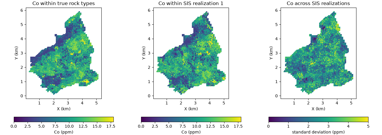
Co within true rock types, Co within SIS realization 1, Co across SIS realizations

within the true rock types, Co drops at each argovian contact and averages 5.45 ppm on argovian. within the SIS rock types the contacts move from one realization to the next, so the lean argovian Co spreads over its uncertain margin: the true argovian averages 7.20 ppm. where SIS is unsure of argovian (a third of the nodes), the spread of Co across realizations is 2.87 ppm against 2.07 ppm with the domains fixed.

Total running time of the script: ( 0 minutes 0.724 seconds)

Download Python source code: example_07_08.py

Download Jupyter notebook: example_07_08.ipynb

Gallery generated by mkdocs-gallery