Note
Click here to download the full example code
external drift kriging
copper grades from the soil geochemistry survey (the dataset of
despiking) correlate weakly with the magnetics and elevation of
the covariates grid. ExternalDriftKriging drapes those covariates onto the samples and kriges copper with them as an
extra drift, in one system with the usual constant term. ordinary kriging on the same grid is the comparison.
import sys
from pathlib import Path

HERE = Path(__file__).parent if "__file__" in globals() else Path.cwd()
sys.path.insert(0, str(HERE.parents[1]))
import boitata as bt
import matplotlib.pyplot as plt
import numpy as np
from common import ACCENT, INK, map_axes, save

data = bt.datasets.soil_geochemistry_survey()
samples, covariates = data["samples"], data["covariates"]
BlockModel.sample reads the cell under each sample, draping MAG_NT and ELEVATION_M onto the samples as two new
columns.
samples = samples.with_columns(
    {c: covariates.sample(samples.coords[:, :2], c) for c in ("MAG_NT", "ELEVATION_M")}
)
print(
    f"correlation with Cu: magnetics {np.corrcoef(samples['CU_PPM'], samples['MAG_NT'])[0, 1]:.2f}, "
    f"elevation {np.corrcoef(samples['CU_PPM'], samples['ELEVATION_M'])[0, 1]:.2f}"
)
Out:
correlation with Cu: magnetics 0.23, elevation 0.33
a single spherical structure fitted to the omnidirectional experimental variogram of copper.
xy, cu = samples.coords, samples["CU_PPM"]
model = bt.experimental_variogram(xy, cu, 200.0, 2500.0).fit(["spherical"], weighting="count/gamma")
search = bt.Search(radius=2000.0, max_samples=24, min_samples=4)
print(model)
Out:
Variogram(nugget=332.2180833057617, structures=[Structure("spherical", sill=1304.5267825034605, range=1783.5147070962437)], rotation=(0.0, 0.0, 0.0), ratios=(1.0, 1.0))
ExternalDriftKriging takes the drift column names at fit (read off samples) and again at predict (read off
covariates, which already carries them); OrdinaryKriging ignores the covariates.
inside = covariates["INSIDE"] == 1
ok = bt.OrdinaryKriging(model, search).fit(samples, "CU_PPM").predict(covariates)
edk = (
    bt.ExternalDriftKriging(model, search, ["MAG_NT", "ELEVATION_M"])
    .fit(samples, "CU_PPM")
    .predict(covariates)
)
ok, edk = (np.where(inside, e, np.nan) for e in (ok, edk))
print(f"mean: ordinary {np.nanmean(ok):.1f}, external drift {np.nanmean(edk):.1f} ppm")
print(f"correlation between the two maps: {np.corrcoef(ok[inside], edk[inside])[0, 1]:.3f}")
Out:
mean: ordinary 54.8, external drift 54.3 ppm
correlation between the two maps: 0.970
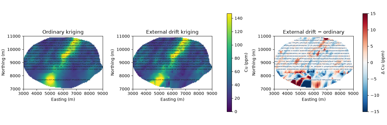
the two maps agree where covariates are flat and pull apart where magnetics or elevation depart from the neighborhood mean. the drift nudges the estimate up in high-magnetics, high-elevation ground even far from any sample, which ordinary kriging's constant mean cannot do.
low, high = covariates.bounds
extent = (low[0], high[0], low[1], high[1])
vmax = np.nanpercentile(np.r_[ok, edk], 98)
fig, axes = plt.subplots(1, 3, figsize=(13, 4.2), layout="constrained")
for ax, image, title in ((axes[0], ok, "Ordinary kriging"), (axes[1], edk, "External drift kriging")):
    im = ax.imshow(covariates.grid(image)[0], origin="lower", extent=extent, vmin=0, vmax=vmax)
    ax.scatter(samples.x, samples.y, s=2, color=INK, linewidths=0)
    map_axes(ax, title)
fig.colorbar(im, ax=axes[:2], shrink=0.8, label="Cu (ppm)")
diff = ax = axes[2]
d = ax.imshow(covariates.grid(edk - ok)[0], origin="lower", extent=extent, cmap="RdBu_r", vmin=-15, vmax=15)
ax.scatter(samples.x, samples.y, s=2, color=ACCENT, linewidths=0)
map_axes(ax, "External drift − ordinary")
fig.colorbar(d, ax=diff, shrink=0.8, label="Δ Cu (ppm)")
save(fig, "maps")
cross_validate and weight declustering do not support external-drift kriging yet: each held-out point or target
would need its own covariate row, which those two do not carry through.
Total running time of the script: ( 0 minutes 0.317 seconds)
Download Python source code: example_06_04.py