grade shells¶

an implicit model fits a scalar field to the data and takes a surface as one of its level sets, so you skip digitizing outlines section by section. here the drill-hole composites of the iron formation plateau give a Fe ≥ 60 % shell, compared with the supplied high_grade.stl solid.

import sys
from pathlib import Path

HERE = Path(__file__).parent if "__file__" in globals() else Path.cwd()
sys.path.insert(0, str(HERE.parents[1]))

import boitata as bt
import matplotlib.pyplot as plt
import numpy as np
from common import ACCENT, GRAY, HIGHLIGHT, LIGHT, save

with cutoff=60 each composite gets the code +1 at or above the cutoff and −1 below, so the shell is the zero level of the field. a radial basis function (RBF) interpolates the codes exactly by solving one dense system, whose cost grows with the cube of the sample count, so 12 m composites keep it to a few thousand samples. the plateau's layers are flat, so a second RBF shrinks distances across them (ratios: vertical ranges a fifth of the horizontal). a sparse gaussian process (GP) smooths through the codes and learns its own ranges.

data = bt.datasets.iron_formation_plateau()
holes = bt.Drillholes.from_tables(data)
composites = holes.composite(12.0, ["FE_PCT"]).drop_null("FE_PCT")
xyz, fe = composites.coords, composites["FE_PCT"]
code = np.where(fe >= 60, 1.0, -1.0)
print(f"{len(xyz)} composites, {(code > 0).sum()} at or above 60 % Fe")

models = {
    "RBF": bt.ImplicitModel("rbf", degree=0),
    "RBF, flat": bt.ImplicitModel("rbf", degree=0, rotation=(0, 0, 0), ratios=(1, 0.2)),
    "GP": bt.ImplicitModel("gp", degree=0),
}
for name, model in models.items():
    model.fit(xyz, fe, cutoff=60)
    print(f"{name:>9}: {np.mean(np.sign(model.predict(xyz)) == code):.1%} of composites on their side")
print(f"GP ranges {[round(r) for r in models['GP'].report['lengthscales']]} m")

Out:

3437 composites, 658 at or above 60 % Fe
      RBF: 100.0% of composites on their side
RBF, flat: 100.0% of composites on their side
       GP: 87.2% of composites on their side
GP ranges [744, 1475, 262] m

each field goes onto the supplied block model, 25 × 25 × 12 m blocks below topography, and against the solid: the volume of the shell, the share of the solid it covers and the share of its own volume outside the solid. the composites score the solid too.

solid, blocks = data["high_grade"], data["block_model"]
in_solid = solid.contains(blocks.coords)
on_side = np.mean(np.where(solid.contains(xyz), 1, -1) == code)
print(f"    solid: {solid.volume / 1e6:5.1f} Mm3, {on_side:.1%} of composites on their side")
for name, model in models.items():
    inside = model.predict(blocks) > 0
    print(
        f"{name:>9}: {blocks.volumes[inside].sum() / 1e6:5.1f} Mm3, "
        f"covers {blocks.volumes[inside & in_solid].sum() / blocks.volumes[in_solid].sum():.0%} of the solid, "
        f"{(inside & ~in_solid).sum() / inside.sum():.0%} outside it"
    )

Out:

    solid:  75.5 Mm3, 91.4% of composites on their side
      RBF:  57.0 Mm3, covers 56% of the solid, 29% outside it
RBF, flat:  67.4 Mm3, covers 65% of the solid, 29% outside it
       GP:  47.7 Mm3, covers 50% of the solid, 23% outside it

both RBFs honor each code, yet they cover only 56 % and 65 % of the solid, and the solid leaves 8.6 % of the composites on the wrong side: a cutoff on Fe and a solid interpreted around the shallow friable hematite are two different surfaces. flattening the RBF adds a tenth of the solid at no cost in spill. the GP explains an eighth of the codes as noise and returns a smooth sheet. on an east-west section through the high-grade composites, at true scale, with the trace of the solid in black and topography as a thin line:

northing = 25 * round(np.median(xyz[code > 0, 1]) / 25)
x, z = np.meshgrid(np.arange(44000, 46100, 5.0), np.arange(300, 720, 3.0))
section = np.c_[x.ravel(), np.full(x.size, northing), z.ravel()]
topography = data["topography"]
row = np.isclose(topography.y, northing, atol=12.5)
ground = np.interp(x[0], topography.x[row], topography["Z"][row])
plane = ((0, northing, 0), 90, 90)
fig, axes = plt.subplots(3, 1, figsize=(12, 8.5), layout="constrained", sharex=True)
for ax, (name, model) in zip(axes, models.items(), strict=True):
    field = np.where(z <= ground, model.predict(section).reshape(x.shape), np.nan)
    ax.contourf(x, z, field, levels=[0, np.inf], colors=[LIGHT])
    ax.contour(x, z, field, levels=[0], colors=[ACCENT], linewidths=1.2)
    ax.plot(x[0], ground, color=GRAY, lw=0.8)
    style = {"plane": plane, "thickness": 50, "ax": ax}
    bt.plot.slab(xyz[code < 0], s=6, color=GRAY, label="Fe < 60 %", meshes=solid, **style)
    bt.plot.slab(xyz[code > 0], s=6, color=HIGHLIGHT, label="Fe ≥ 60 %", **style)
    ax.set(title=f"{name}, northing {northing:.0f} m", xlim=(x[0, 0], x[0, -1]), ylim=(z[0, 0], z[-1, 0]))
    if ax is not axes[-1]:
        ax.set_xlabel("")
axes[0].legend(loc="lower right", title="composites within 25 m", ncol=2)
save(fig, "section")

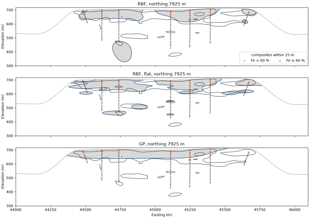
RBF, northing 7925 m, RBF, flat, northing 7925 m, GP, northing 7925 m

the isotropic RBF grows a round body around one deep high-grade composite; the flat one keeps it a thin pod, as the solid does. isosurface triangulates the zero level at the centroids of the block model and treats blocks outside its mask, here those above topography, as outside the shell. with closed=True it caps the shell where it leaves the blocks, at the grid's faces and under topography, so the shell bounds a volume close to that of the blocks inside.

shell = models["RBF, flat"].isosurface(blocks, closed=True)
inside = models["RBF, flat"].predict(blocks) > 0
print(
    f"flat RBF shell: {len(shell.triangles):,} triangles, closed {shell.is_closed}, {shell.volume / 1e6:.1f} Mm3; "
    f"blocks inside {blocks.volumes[inside].sum() / 1e6:.1f} Mm3"
)

Out:

flat RBF shell: 74,788 triangles, closed True, 64.6 Mm3; blocks inside 67.4 Mm3

Total running time of the script: ( 0 minutes 18.063 seconds)

Download Python source code: example_11_01.py

Download Jupyter notebook: example_11_01.ipynb

Gallery generated by mkdocs-gallery