Note
Click here to download the full example code
swaths
phosphate concentrated by weathering, drilled by 217 RC and 34 diamond holes through soil (SOIL), an aluminous horizon (ALU), the oxidized ore (OXI), saprolite (SAP) and fresh rock (ROCK). a swath is the mean grade in slices along one direction. a trend in the data shows up as a slope, and the same call on a block model checks the estimate for local bias (model checks).
import sys
from pathlib import Path

HERE = Path(__file__).parent if "__file__" in globals() else Path.cwd()
sys.path.insert(0, str(HERE.parents[1]))
import boitata as bt
import matplotlib.pyplot as plt
from common import save

data = bt.datasets.phosphate_weathering_profile()
intervals = bt.merge_intervals(data["assays"], data["horizons"])
samples = bt.Drillholes(data["collars"], data["surveys"], intervals).samples()
stats = bt.describe_by("P2O5_PCT", "HORIZON", data=samples)
for name, n, mean in zip(stats["category"], stats["n"], stats["mean"], strict=True):
    print(f"{name:<5}{n:>6.0f} samples, mean P2O5 {mean:5.2f} %")
length = samples["TO"] - samples["FROM"]
print(f"sample length {length.min():.1f} to {length.max():.1f} m")
Out:
ALU    1042 samples, mean P2O5  4.92 %
OXI    1432 samples, mean P2O5 12.92 %
ROCK   1316 samples, mean P2O5  5.09 %
SAP     998 samples, mean P2O5  9.07 %
SOIL    251 samples, mean P2O5  1.94 %
all    5039 samples, mean P2O5  7.91 %
sample length 0.5 to 6.6 m
the ore is the OXI horizon, with SAP below it half as rich. swath bins the samples in slices of a given width along
axis ("x", "y", "z") or any azimuth, weighted here by sample length since the samples run from 0.5 to 6.6 m.
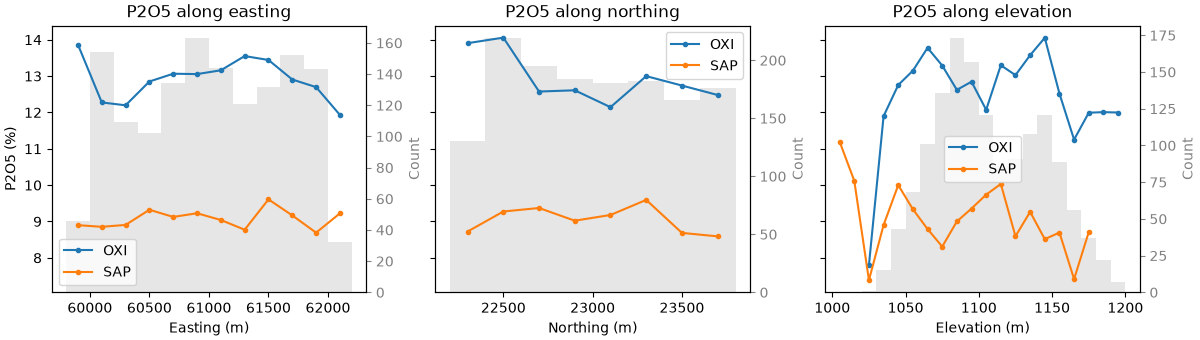
plot.swath draws several swaths on one axis, with the counts of the first as bars. the slices are 200 m along
easting and northing and 10 m in elevation, one line per horizon.
horizons = ["OXI", "SAP"]
fig, axes = plt.subplots(1, 3, figsize=(12, 3.4), layout="constrained", sharey=True)
for ax, axis, width, label in zip(
    axes, "xyz", [200.0, 200.0, 10.0], ["Easting", "Northing", "Elevation"], strict=True
):
    swaths = []
    for name in horizons:
        horizon = samples.filter(samples["HORIZON"] == name)
        length = horizon["TO"] - horizon["FROM"]
        swaths.append(bt.swath(horizon, "P2O5_PCT", width, axis=axis, weights=length))
    bt.plot.swath(swaths, labels=horizons, ax=ax)
    ax.set(title=f"P2O5 along {label.lower()}", xlabel=f"{label} (m)")
    ax.set_ylabel("")
    for name, swath in zip(horizons, swaths, strict=True):
        mean = swath["mean"][swath["n"] >= 30]
        print(
            f"{name} along {label.lower()}: {mean.min():.1f} to {mean.max():.1f} %, slices of 30 samples or more"
        )
axes[0].set_ylabel("P2O5 (%)")
save(fig, "swaths")
Out:
OXI along easting: 11.9 to 13.9 %, slices of 30 samples or more
SAP along easting: 8.7 to 9.6 %, slices of 30 samples or more
OXI along northing: 12.1 to 14.1 %, slices of 30 samples or more
SAP along northing: 8.6 to 9.6 %, slices of 30 samples or more
OXI along elevation: 11.3 to 14.1 %, slices of 30 samples or more
SAP along elevation: 7.4 to 10.0 %, slices of 30 samples or more
within each horizon the swaths are flat. OXI stays between 11.9 and 14.1 % along easting and northing and SAP between 8.6 and 9.6 %, about the noise that a hundred-odd samples per slice leave. the step between the two lines is much larger than any slope along them, so the horizon sets the grade: estimate each horizon on its own samples, with no trend. in elevation the lines are noisier because the horizons follow the rolling topography, and one slice of elevation cuts OXI on a hill and SAP in a valley. the slices at the ends hold few samples, and the bars tell you how far to trust them.
Total running time of the script: ( 0 minutes 2.105 seconds)
Download Python source code: example_03_09.py