variogram fitting¶

you fit an anisotropic nested spherical model of V to directional experimental variograms along and across the direction of greatest continuity (experimental variograms builds them), then to all directions at once with fit_directional.

import sys
from pathlib import Path

HERE = Path(__file__).parent if "__file__" in globals() else Path.cwd()
sys.path.insert(0, str(HERE.parents[1]))

import boitata as bt
import matplotlib.pyplot as plt
import numpy as np
from common import ACCENT, GRAY, HIGHLIGHT, INK, save

samples = bt.datasets.walker_lake()
xy, v = samples.coords, samples["V"]
lag, max_lag = 10.0, 120.0

the variogram map picks the major axis, the direction with the longest fitted range.

vmap = bt.variogram_map(xy, v, lag, max_lag)
angle = vmap.angles[np.nanargmax(vmap.ranges)]
azimuth = (90 - np.degrees(angle)) % 180

fit along and across the major axis. weighting each lag by N(h)/γ(h)² lets the few short-lag pairs steer the fit near the origin, where the nugget and the short ranges are decided.

major = bt.experimental_variogram(xy, v, lag, max_lag, azimuth=azimuth)
minor = bt.experimental_variogram(xy, v, lag, max_lag, azimuth=azimuth + 90)
weighting = "count/gamma"
single = major.fit("spherical", weighting=weighting)
along = major.fit(["spherical", "spherical"], weighting=weighting)
print(single, along, minor.fit(["spherical", "spherical"], weighting=weighting), sep="\n")

Out:

Variogram(nugget=31621.585548875744, structures=[Structure("spherical", sill=61718.46041352483, range=72.70834074501036)], rotation=(0.0, 0.0, 0.0), ratios=(1.0, 1.0))
Variogram(nugget=14993.35122178715, structures=[Structure("spherical", sill=25261.581155025888, range=19.578360959734756), Structure("spherical", sill=53364.6905008533, range=80.65434681410247)], rotation=(0.0, 0.0, 0.0), ratios=(1.0, 1.0))
Variogram(nugget=23378.007796960097, structures=[Structure("spherical", sill=0, range=2.5), Structure("spherical", sill=68505.76265942639, range=23.87806723833898)], rotation=(0.0, 0.0, 0.0), ratios=(1.0, 1.0))

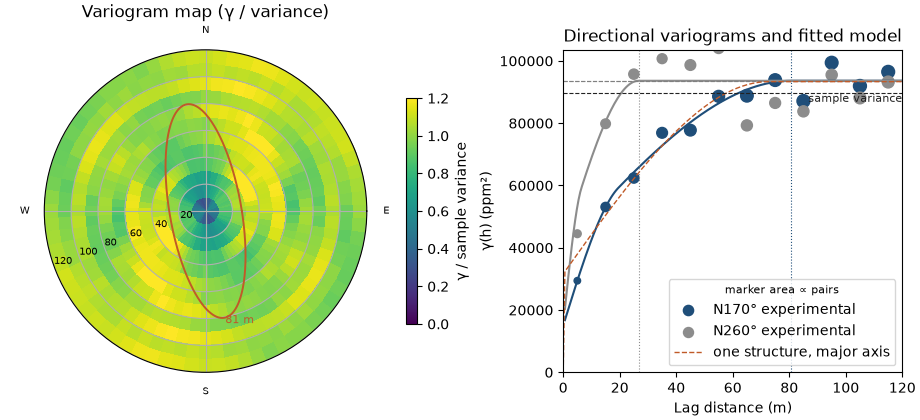
along the major axis γ climbs to two thirds of the sill within 25 m, then rises slowly to about 80 m: two scales of continuity. one structure (dashed below) splits the difference, overshoots the first lags and puts a third of the sill in the nugget. two nested spherical structures follow both scales and halve the nugget. across the axis the short structure takes no sill: γ reaches the sill by 25 m, and the data support one structure.

the structures share one anisotropy. fitting the minor direction with the nugget and sills fixed at their major-axis values moves only its ranges; the long structure, with two thirds of the sill, sets the minor/major ratio. rotation is azimuth, dip, rake in degrees; ratios are semi-major/major and minor/major ranges.

sills = [s.sill for s in along.structures]
across = minor.fit(["spherical", "spherical"], weighting=weighting, nugget=along.nugget, sills=sills)
a_major = along.structures[-1].range
ratio = min(across.structures[-1].range / a_major, 1.0)
model = along.with_anisotropy(rotation=(azimuth, 0, 0), ratios=(ratio, 1.0))
print(across)
print(model)

Out:

Variogram(nugget=14993.35122178715, structures=[Structure("spherical", sill=25261.581155025888, range=12.181126916520325), Structure("spherical", sill=53364.6905008533, range=26.669590607377888)], rotation=(0.0, 0.0, 0.0), ratios=(1.0, 1.0))
Variogram(nugget=14993.35122178715, structures=[Structure("spherical", sill=25261.581155025888, range=19.578360959734756), Structure("spherical", sill=53364.6905008533, range=80.65434681410247)], rotation=(170.0, 0.0, 0.0), ratios=(0.33066526059466755, 1.0))

the ellipse on the map is the model range in each direction:

variance = v.var()
fig = plt.figure(figsize=(9.2, 4.2), layout="constrained")
a = fig.add_subplot(1, 2, 1, projection="polar")
gamma = np.where(vmap.counts >= 30, vmap.gammas, np.nan)
step = vmap.angles[1] - vmap.angles[0]
theta = np.r_[vmap.angles, vmap.angles + np.pi, 2 * np.pi] - step / 2
radius = np.r_[vmap.lags - lag / 2, vmap.lags[-1] + lag / 2]
mesh = a.pcolormesh(theta, radius, np.vstack([gamma, gamma]).T / variance, vmin=0, vmax=1.2, shading="flat")
t = np.linspace(0, 2 * np.pi, 361)
direction = np.radians(90 - azimuth)
a_minor = a_major * ratio
ellipse = a_major * a_minor / np.hypot(a_minor * np.cos(t - direction), a_major * np.sin(t - direction))
a.plot(t, ellipse, color=HIGHLIGHT, lw=1.4)
a.text(direction, a_major * 1.05, f"{a_major:.0f} m", color=HIGHLIGHT, fontsize=8)
a.set_rlim(0, radius[-1])
a.set_xticks(np.radians([0, 90, 180, 270]), ["E", "N", "W", "S"])
a.set_rlabel_position(200)
a.tick_params(labelsize=7)
a.set_title("Variogram map (γ / variance)")
fig.colorbar(mesh, ax=a, shrink=0.7, label="γ / sample variance")

b = fig.add_subplot(1, 2, 2)
for exp, color, az, rng in ((major, ACCENT, azimuth, a_major), (minor, GRAY, azimuth + 90, a_minor)):
    bt.plot.variogram(
        exp, variogram=model, direction=(az, 0), ax=b, color=color, label=f"N{az % 360:.0f}° experimental"
    )
    b.axvline(rng, color=color, lw=0.8, ls=":")
h = np.linspace(0, max_lag, 200)
b.plot(h, single.gamma(h), color=HIGHLIGHT, lw=1, ls="--", label="one structure, major axis")
b.axhline(variance, color=INK, lw=0.8, ls="--")
b.text(max_lag, variance, "sample variance", va="top", ha="right", color=INK, fontsize=8)
b.set_xlim(0, max_lag)
b.set_ylim(bottom=0)
b.set_title("Directional variograms and fitted model")
b.set_xlabel("Lag distance (m)")
b.set_ylabel("γ(h) (ppm²)")
b.legend(loc="lower right", title="marker area ∝ pairs", title_fontsize=8)
save(fig, "variogram")

Variogram map (γ / variance), Directional variograms and fitted model

Variogram.fit_directional fits one anisotropic model to experimental variograms in many directions at once: azimuth, range ratio, ranges, sills and nugget together, with the ranges along the major axis. the directions here are horizontal, every 22.5°, so the fit is 2D: dip, rake and the minor/major ratio stay 0, 0 and 1.

azimuths = np.arange(0, 180, 22.5)
directional = [bt.experimental_variogram(xy, v, lag, max_lag, azimuth=a) for a in azimuths]
joint = bt.Variogram.fit_directional(
    directional, [(a, 0) for a in azimuths], ["spherical", "spherical"], weighting=weighting
)
print(joint)

Out:

Variogram(nugget=16458.263904055566, structures=[Structure("spherical", sill=39532.539054973735, range=36.61762520915539), Structure("spherical", sill=39110.929672733, range=115)], rotation=(161.46015029654865, 0.0, 0.0), ratios=(0.33583545063941, 1.0))

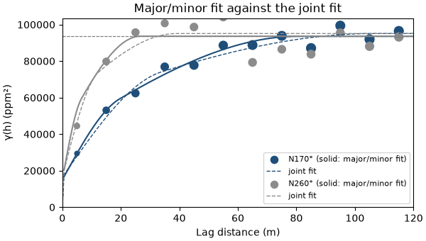
the joint fit puts the major axis at N161°, nine degrees off the map's pick, with the same one-third ratio. its long range stops at 115 m, the largest lag, where free ranges are capped unless ranges bounds them. spread over all eight directions, it fits the major and minor axes worse than the fits made along them: the dashed curves fall below the short lags on both. %%

fig, ax = plt.subplots(figsize=(6, 3.4), layout="constrained")
origin = np.zeros((h.size, 3))
for exp, color, az in ((major, ACCENT, azimuth), (minor, GRAY, azimuth + 90)):
    bt.plot.variogram(
        exp,
        variogram=model,
        direction=(az, 0),
        ax=ax,
        color=color,
        label=f"N{az % 360:.0f}° (solid: major/minor fit)",
    )
    unit = np.array([np.sin(np.radians(az)), np.cos(np.radians(az)), 0])
    ax.plot(h, joint.gamma_between(origin, h[:, None] * unit), color=color, lw=1, ls="--", label="joint fit")
ax.set_xlim(0, max_lag)
ax.set_title("Major/minor fit against the joint fit")
ax.set_xlabel("Lag distance (m)")
ax.set_ylabel("γ(h) (ppm²)")
ax.legend(loc="lower right", fontsize=8)
save(fig, "joint")