Note
Click here to download the full example code
declustering
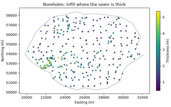
a coal seam drilled on a regular mesh, then infilled where the seam is thick. the infill holes over-represent thick coal, so the plain mean of the boreholes overstates the thickness of the seam. declustering weights each hole by the area it stands for: cell declustering by the number of holes sharing its cell, polygonal declustering by the area nearer to it than to any other hole.
import sys
from pathlib import Path

HERE = Path(__file__).parent if "__file__" in globals() else Path.cwd()
sys.path.insert(0, str(HERE.parents[1]))
import boitata as bt
import matplotlib.pyplot as plt
import numpy as np
from common import ACCENT, GRAY, INK, map_axes, save

data = bt.datasets.coal_seam_thickness()
holes, lease = data["boreholes"], data["boundary"]
thickness = holes["THICKNESS_M"]
x, y = holes.x, holes.y
print(f"{len(holes)} holes, mean thickness {thickness.mean():.2f} m")

fig, ax = plt.subplots(figsize=(7, 4.4), layout="constrained")
drawn = ax.scatter(x, y, c=thickness, s=14, edgecolors=INK, linewidths=0.3)
ax.plot(*lease.coords[:, :2].T, color=GRAY, lw=0.8)
fig.colorbar(drawn, ax=ax, shrink=0.8, label="Thickness (m)")
map_axes(ax, "Boreholes: infill where the seam is thick")
save(fig, "holes")
Out:
295 holes, mean thickness 2.23 m
cell declustering
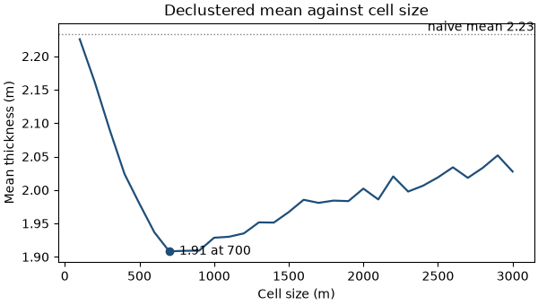
each hole gets the inverse of the number of holes in its cell. too small a cell holds one hole and changes nothing;
too large a cell holds the whole lease. in between, when the infill targets high values, the declustered mean dips.
cell_declustering scans cell sizes, averages each over 25 grid origins, and keeps the size with the lowest mean. the
weights average 1.
cell = bt.cell_declustering(holes, "THICKNESS_M", sizes=np.arange(100.0, 3100.0, 100.0))
print(
    f"cell size {cell.cell_size:.0f} m, declustered mean {np.average(thickness, weights=cell.weights):.2f} m"
)
print(f"scanned mean at that size {cell.means[cell.sizes == cell.cell_size][0]:.2f} m")

fig, ax = plt.subplots(figsize=(6, 3.4), layout="constrained")
bt.plot.declustering(cell, naive=thickness.mean(), ax=ax, color=ACCENT, lw=1.6)
ax.set(title="Declustered mean against cell size", xlabel="Cell size (m)", ylabel="Mean thickness (m)")
save(fig, "cell_sizes")
Out:
cell size 700 m, declustered mean 1.91 m
scanned mean at that size 1.91 m
the mean falls from 100 m cells, which hold about one hole each, to a flat minimum between 700 and 900 m. it then rises slowly as the cells grow to hold mesh and infill holes alike. choosing the cell size is a judgment, and the minimum guides it only when you know the infill targets high values, as here. the curve averages 25 grid origins, while the returned weights come from one origin at the corner of the data, so their mean (the dot) sits a little above the curve.
polygonal declustering
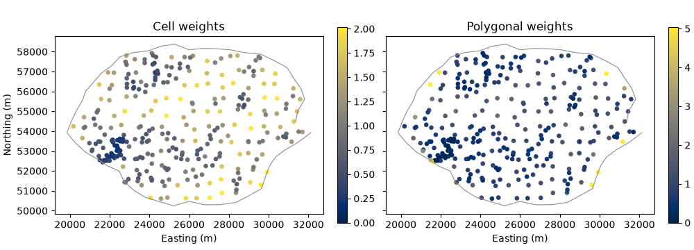
polygon_declustering weights each hole by the area of the grid nodes nearest to it, over the bounding box of the
holes. it needs no cell size, but the holes on the edge take all the area out to the box, and the box differs from the
lease.
polygon = bt.polygon_declustering(holes, "THICKNESS_M")
print(f"polygonal declustered mean {np.average(thickness, weights=polygon.weights):.2f} m")
fig, axes = plt.subplots(1, 2, figsize=(10, 3.6), layout="constrained", sharey=True)
for ax, result, name in zip(axes, [cell, polygon], ["Cell", "Polygonal"], strict=True):
    w = result.weights
    drawn = ax.scatter(x, y, c=w, s=14, cmap="cividis", vmin=0, vmax=np.percentile(w, 98))
    ax.plot(*lease.coords[:, :2].T, color=GRAY, lw=0.8)
    map_axes(ax, f"{name} weights")
    fig.colorbar(drawn, ax=ax, shrink=0.8)
axes[1].set_ylabel("")
save(fig, "weights")
Out:
polygonal declustered mean 1.95 m
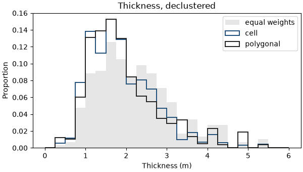
both methods give the infill holes small weights and the sparse mesh large ones, and they agree on the declustered mean. the largest polygonal weights sit on the edge of the drilling, where the box reaches past the lease. the declustered histograms shift toward thin coal.
bins = np.linspace(0, np.ceil(thickness.max()), 25)
fig, ax = plt.subplots(figsize=(6, 3.4), layout="constrained")
ax.hist(thickness, bins, weights=np.full(len(holes), 1 / len(holes)), color="#e6e6e6", label="equal weights")
for result, color, label in [(cell, ACCENT, "cell"), (polygon, INK, "polygonal")]:
    ax.hist(
        thickness,
        bins,
        weights=result.weights / len(holes),
        histtype="step",
        color=color,
        lw=1.4,
        label=label,
    )
ax.set(title="Thickness, declustered", xlabel="Thickness (m)", ylabel="Proportion")
ax.legend()
save(fig, "histograms")
these weights describe the data: histograms, statistics per domain, top cuts and the target of a normal-score transform. weight declustering derives declustering weights from estimation weights, from what each hole contributes to estimating the whole lease.
Total running time of the script: ( 0 minutes 0.579 seconds)
Download Python source code: example_03_03.py