Note
Click here to download the full example code
sequential indicator simulation
sequential indicator simulation (SIS) draws categories. it visits the nodes along a random path, krigs the indicator of each category with its own variogram from the samples and the nodes already drawn, and draws a category from those probabilities. each realization is one possible rock-type map; over many realizations, the frequency of each category at a node is its probability. categorical indicator kriging estimates such probabilities without simulating.
import sys
from pathlib import Path

HERE = Path(__file__).parent if "__file__" in globals() else Path.cwd()
sys.path.insert(0, str(HERE.parents[1]))
import boitata as bt
import matplotlib.pyplot as plt
import numpy as np
from common import ACCENT, GRAY, save
rock types
jura's rock types are known at each node of the prediction grid, so you can compare simulated maps with the real
geology. a Categories scheme names the five types and gives each a color: encode turns labels into the codes 0
to 4 that SIS takes, and shares gives their proportions.
jura = bt.datasets.jura()
train, grid = jura["prediction"], jura["grid"]
names = ["Argovian", "Kimmeridgian", "Sequanian", "Portlandian", "Quaternary"]
rock_types = bt.Categories(names, colors=["#1f4e79", "#6f9fc9", "#c9d9ea", "#c05a28", "#8c8c8c"])
rock = rock_types.encode(train["Rock"]).astype(int)
true_rock = rock_types.encode(grid["Rock"]).astype(int)
print(f"{len(rock)} samples, {len(true_rock)} grid nodes")
print(f"{'':<13}{'samples':>8}{'share':>7}{'true grid':>11}")
for k, name in enumerate(names):
    print(f"{name:<13}{np.sum(rock == k):8d}{np.mean(rock == k):7.2f}{np.mean(true_rock == k):11.2f}")
Out:
259 samples, 5957 grid nodes
              samples  share  true grid
Argovian           53   0.20       0.20
Kimmeridgian       85   0.33       0.34
Sequanian          63   0.24       0.27
Portlandian         3   0.01       0.05
Quaternary         55   0.21       0.13
indicator variograms
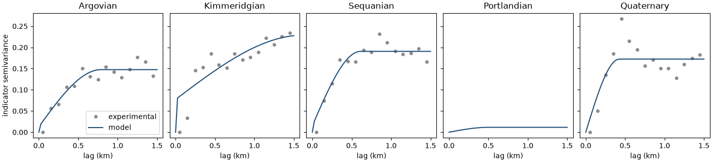
each rock type gets the variogram of its indicator, 1 inside the type and 0 outside. portlandian has too few samples for an experimental variogram, so it gets a short spherical model with the indicator's variance as sill.
experimental, variograms = [], []
for k in range(5):
    indicator = (rock == k).astype(float)
    if indicator.sum() >= 5:
        experimental.append(bt.experimental_variogram(train.coords, indicator, 0.1, 1.5))
        variograms.append(experimental[-1].fit("spherical"))
    else:
        experimental.append(None)
        variograms.append(bt.Variogram([("spherical", indicator.var(), 0.5)]))
for name, v in zip(names, variograms):
    s = v.structures[0]
    print(f"{name:<13}nugget {v.nugget:.3f}, sill {s.sill:.3f}, range {s.range:.2f} km")
Out:
Argovian     nugget 0.013, sill 0.135, range 0.79 km
Kimmeridgian nugget 0.077, sill 0.152, range 1.62 km
Sequanian    nugget 0.015, sill 0.176, range 0.61 km
Portlandian  nugget 0.000, sill 0.011, range 0.50 km
Quaternary   nugget 0.000, sill 0.172, range 0.43 km
h = np.linspace(0, 1.5, 61)
fig, axes = plt.subplots(1, 5, figsize=(14, 3.2), layout="constrained", sharey=True)
for ax, name, e, v in zip(axes, names, experimental, variograms):
    if e is not None:
        ax.plot(e.lags, e.gammas, "o", color=GRAY, ms=4, label="experimental")
    ax.plot(h, v.gamma(h), color=ACCENT, label="model")
    ax.set(title=name, xlabel="lag (km)")
axes[0].set_ylabel("indicator semivariance")
axes[0].legend(loc="lower right")
save(fig, "variograms")
realizations
simulate returns a summary over n realizations: probabilities holds each type's frequency, one row per node,
most_likely the most frequent type, and entropy, scaled to [0, 1], how evenly the realizations disagree.
keep=True keeps the maps.
sis = bt.SIS(variograms, bt.Search(radius=1.5, max_samples=16)).fit(train, rock)
summary = sis.simulate(grid, n=20, seed=3, keep=True)
maps = summary.realizations
shares = np.array([rock_types.shares(m) for m in maps])
print(f"{'':<13}{'true grid':>10}{'mean':>7}{'min':>7}{'max':>7}")
for k, name in enumerate(names):
    print(
        f"{name:<13}{np.mean(true_rock == k):10.2f}{shares[:, k].mean():7.2f}"
        f"{shares[:, k].min():7.2f}{shares[:, k].max():7.2f}"
    )
match = np.mean(maps == true_rock, axis=1)
print(f"a realization matches the true rock type at {match.min():.0%} to {match.max():.0%} of the nodes")
print(
    f"the most likely type matches at {np.mean(summary.most_likely == true_rock):.0%}; "
    f"mean entropy {summary.entropy.mean():.2f}"
)
Out:
              true grid   mean    min    max
Argovian           0.20   0.16   0.14   0.19
Kimmeridgian       0.34   0.44   0.39   0.49
Sequanian          0.27   0.24   0.20   0.28
Portlandian        0.05   0.02   0.01   0.03
Quaternary         0.13   0.14   0.12   0.16
a realization matches the true rock type at 53% to 60% of the nodes
the most likely type matches at 64%; mean entropy 0.38
cmap, norm = bt.plot.category_colors(rock_types)
xy = grid.coords[:, :2].T
fig, axes = plt.subplots(2, 3, figsize=(12, 9.5), layout="constrained")
categorical = [(true_rock, "True rock types"), (maps[0], "Realization 1"), (maps[1], "Realization 2")]
for ax, (cats, title) in zip(axes[0], categorical):
    ax.scatter(*xy, c=cats, cmap=cmap, norm=norm, s=7, marker="s", linewidths=0)
    ax.set_title(title)
axes[1, 0].scatter(*xy, c=summary.most_likely, cmap=cmap, norm=norm, s=7, marker="s", linewidths=0)
axes[1, 0].set_title("Most likely over 20 realizations")
for ax, values, title, label, color in (
    (axes[1, 1], summary.probabilities[:, 0], "P(Argovian)", "probability", "cividis"),
    (axes[1, 2], summary.entropy, "Entropy", "entropy", "Greys"),
):
    im = ax.scatter(*xy, c=values, s=7, marker="s", linewidths=0, vmin=0, vmax=1, cmap=color)
    ax.set_title(title)
    fig.colorbar(im, ax=ax, shrink=0.8, orientation="horizontal", label=label)
for ax in axes.flat:
    ax.set_aspect("equal")
    ax.set(xlabel="X (km)", ylabel="Y (km)")
bt.plot.category_legend(rock_types, fig, loc="outside lower center", ncol=5)
save(fig, "realizations")
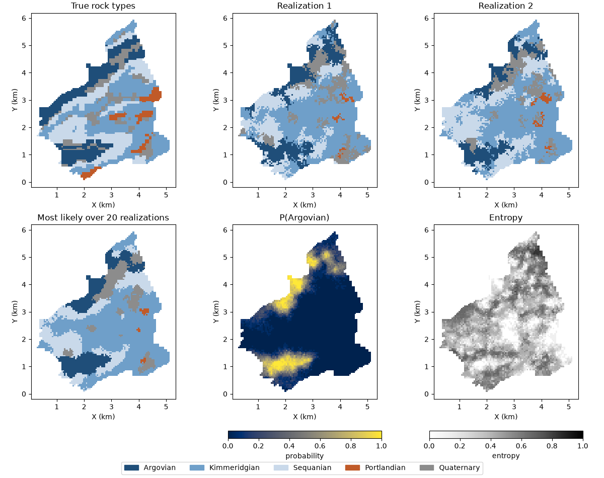
each realization matches the true rock type at 53 % to 60 % of the nodes, and two realizations differ wherever the samples leave room. the proportions drift from the samples: kimmeridgian, whose indicator has the longest range, grows to 0.44 on average against 0.33 in the samples, while argovian and portlandian shrink. no realization recovers portlandian's 5 % of the area from 3 of 259 samples. the most likely type matches at 64 %, more than any realization, though it is a smooth estimate and no possible map looks like it. entropy peaks at the contacts and far from the samples.
Total running time of the script: ( 0 minutes 0.939 seconds)
Download Python source code: example_07_06.py