classification¶

resource classes for the blocks of a coal lease, first from the spacing of the boreholes alone, then from the kriging diagnostics of seam thickness together with the spacing. classify applies rules in order, and smooth_classes absorbs isolated blocks into their surroundings.

import sys
from pathlib import Path

HERE = Path(__file__).parent if "__file__" in globals() else Path.cwd()
sys.path.insert(0, str(HERE.parents[1]))

import boitata as bt
import matplotlib.pyplot as plt
import numpy as np
from common import ACCENT, GRAY, INK, LIGHT, save

data = bt.datasets.coal_seam_thickness()
holes, grid, lease = data["boreholes"], data["grid"], data["boundary"]
blocks = grid.filter(grid["INSIDE"] == 1)
xy, thickness = holes.coords, holes["THICKNESS_M"]
print(f"{len(holes)} boreholes, {len(blocks.coords)} blocks of 100 × 100 m inside the lease")

Out:

295 boreholes, 7162 blocks of 100 × 100 m inside the lease

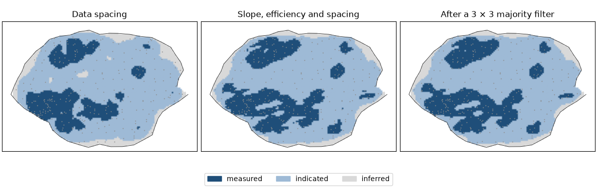
by data spacing¶

data_spacing gives each block the equivalent spacing of the boreholes around it, in plan (data spacing): on a square mesh of spacing s it reads about s. rules apply in order and the first that holds wins; blocks where none holds get the default.

spacing = bt.data_spacing(blocks, holes, None)
rules = [("measured", {"spacing": ("<=", 450)}), ("indicated", {"spacing": ("<=", 700)})]
by_spacing = bt.classify({"spacing": spacing}, rules, default="inferred")
print(f"spacing: median {np.median(spacing):.0f} m, 90th percentile {np.percentile(spacing, 90):.0f} m")

Out:

spacing: median 550 m, 90th percentile 695 m

by kriging diagnostics¶

block kriging with diagnostics=True gives each block its slope of regression and kriging efficiency (kriging diagnostics). the rules add the spacing, so a block needs a well-conditioned estimate and nearby holes.

azimuths = np.arange(0, 180, 45.0)
directional = [bt.experimental_variogram(xy, thickness, 250.0, 4000.0, azimuth=a) for a in azimuths]
model = bt.Variogram.fit_directional(
    directional, [(a, 0) for a in azimuths], ["spherical"], weighting="count/gamma"
)
search = bt.Search(radius=3000, max_samples=16, min_samples=4, rotation=model.rotation, ratios=(0.5, 1.0))
kriging = bt.BlockKriging(model, search, size=(100, 100), discretization=(4, 4, 1)).fit(xy, thickness)
d = kriging.predict(blocks, diagnostics=True)

criteria = {"slope": d["slope"], "efficiency": d["efficiency"], "spacing": spacing}
rules = [
    ("measured", {"slope": (">=", 0.95), "efficiency": (">=", 0.75), "spacing": ("<=", 500)}),
    ("indicated", {"slope": (">=", 0.9), "efficiency": (">=", 0.6), "spacing": ("<=", 800)}),
]
by_kriging = bt.classify(criteria, rules, default="inferred")

smoothing¶

a 3 × 3 majority filter absorbs isolated blocks into their surroundings; cells outside the lease do not vote.

smoothed = bt.smooth_classes(blocks, by_kriging, window=(3, 3, 1))
names = ["measured", "indicated", "inferred"]
print(f"{'':>9} {'spacing':>8} {'kriging':>8} {'smoothed':>9}")
for name in names:
    shares = [np.mean(c == name) for c in (by_spacing, by_kriging, smoothed)]
    print(f"{name:>9}" + "".join(f"{s:>9.1%}" for s in shares))
print(f"{np.mean(smoothed != by_kriging):.1%} of blocks change class in smoothing")

Out:

           spacing  kriging  smoothed
 measured    22.0%    27.3%    27.2%
indicated    68.5%    64.5%    65.0%
 inferred     9.5%     8.1%     7.8%
1.7% of blocks change class in smoothing

spacing alone puts the infill, 22 % of the blocks, in measured, and the lease edge beyond the last holes in inferred. the kriging diagnostics also see how the holes surround a block: measured grows to 27 % and joins the infill patches, while blocks along the edge, with holes on one side only, stay inferred (8.1 % of the lease). the filter changes 1.7 % of the blocks, most of them single blocks and thin fringes.

resource_classes = bt.Categories(names, colors=[ACCENT, "#9ebad6", LIGHT])
cmap, norm = bt.plot.category_colors(resource_classes)
(x0, y0, _), (x1, y1, _) = grid.bounds
extent = (x0, x1, y0, y1)
fig, axes = plt.subplots(1, 3, figsize=(12, 3.8), layout="constrained")
for ax, classes, title in (
    (axes[0], by_spacing, "Data spacing"),
    (axes[1], by_kriging, "Slope, efficiency and spacing"),
    (axes[2], smoothed, "After a 3 × 3 majority filter"),
):
    ax.imshow(
        blocks.grid(resource_classes.encode(classes))[0], origin="lower", extent=extent, cmap=cmap, norm=norm
    )
    ax.plot(*lease.coords[:, :2].T, color=INK, lw=0.6)
    ax.scatter(holes.x, holes.y, s=2, color=GRAY, linewidths=0)
    ax.set(title=title, aspect="equal", xticks=[], yticks=[])
bt.plot.category_legend(resource_classes, fig, loc="outside lower center", ncol=3)
save(fig, "classes")