Note
Click here to download the full example code
capping transform
Capping makes the top cut a pipeline step: fit chooses a cap per domain from the data, transform clips values to
it, and the fitted caps travel with the object to new data, to JSON and to pickle. you either give the cap or let a
rule choose it: a weighted quantile, a target fraction of metal removed, or a target coefficient of variation.
import sys
from pathlib import Path

HERE = Path(__file__).parent if "__file__" in globals() else Path.cwd()
sys.path.insert(0, str(HERE.parents[1]))
import boitata as bt
import matplotlib.pyplot as plt
import numpy as np
from common import ACCENT, GRAY, HIGHLIGHT, save
the quartz-vein composites of top cuts: gold in four veins, V1 to V4, sampled by diamond holes and underground channels, composited to 1 m and declustered in 20 m cells.
data = bt.datasets.vein_gold_grade_control()
intervals = bt.merge_intervals(data["assays"], data["lithology"])
holes = bt.Drillholes(data["collars"], data["surveys"], intervals)
composites = holes.composite(1.0, ["AU_GPT"], domain="LITH", categories=["VEIN"])
quartz = composites.filter(composites["LITH"] == "QV").drop_null("AU_GPT")
weights = bt.cell_declustering(quartz, "AU_GPT", cell_size=20.0).weights
quartz = quartz.with_column("w", weights)
veins = sorted(set(quartz["VEIN"]))
print(f"{len(quartz)} composites in {len(veins)} veins")
Out:
5826 composites in 4 veins
one cap per vein
each rule fits per vein on the declustered composites. the quantile rule caps at the declustered P99, the metal rule
finds the cap that removes 5 % of the metal of each vein, and the CV rule finds the largest cap whose capped
coefficient of variation is 1.5. caps_ and metal_removed_ are dicts by vein.
rules = {
    "P99": bt.Capping(quantile=0.99),
    "5 % metal": bt.Capping(metal_removed=0.05),
    "CV 1.5": bt.Capping(cv=1.5),
}
for rule in rules.values():
    rule.fit("AU_GPT", domain_column="VEIN", weights="w", data=quartz)
print(f"{'vein':<6}" + "".join(f"{name:>11}{'metal (%)':>11}" for name in rules))
for vein in veins:
    row = "".join(f"{r.caps_[vein]:>11.1f}{100 * r.metal_removed_[vein]:>11.2f}" for r in rules.values())
    print(f"{vein:<6}{row}")
Out:
vein          P99  metal (%)  5 % metal  metal (%)     CV 1.5  metal (%)
V1           81.3      10.76      160.6       5.00       48.4      17.07
V2           71.7      15.38      591.8       5.00       48.7      19.38
V3           67.5       0.00       50.5       5.00       54.0       3.97
V4          183.5       0.71      111.6       5.00       52.0      30.36
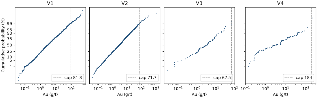
the rules disagree most where the tail is longest. V1 and V2 lose 11 and 15 % of their metal at the P99; holding the loss to 5 % lifts their caps to 161 and 592 g/t, the latter just under the extreme channels of V2. in the small veins the P99 barely cuts: it is the maximum of V3. a CV of 1.5 caps V1 and V2 near 50 g/t and costs them 17 to 19 % of their metal.
the same numbers as top cuts
top cuts read the declustered P99 of each vein off
describe_by and passed it to capping_report. the quantile rule fits the same caps, and its metal_removed_ is the
1 - mean_capped / mean of the report.
capping = rules["P99"]
stats = bt.describe_by("AU_GPT", "VEIN", weights="w", quantiles=[0.99], data=quartz)
top = dict(zip(stats["category"][:-1], stats["P99"][:-1], strict=True))
report = bt.capping_report("AU_GPT", top, domain_column="VEIN", weights="w", data=quartz)
removed = 1 - report["mean_capped"] / report["mean"]
print(f"{'vein':<5}{'P99':>8}{'fitted cap':>12}{'report (%)':>12}{'fitted (%)':>12}")
for k, vein in enumerate(report["domain"][:-1]):
    print(
        f"{vein:<5}{top[vein]:>8.2f}{capping.caps_[vein]:>12.2f}"
        f"{100 * removed[k]:>12.2f}{100 * capping.metal_removed_[vein]:>12.2f}"
    )
Out:
vein      P99  fitted cap  report (%)  fitted (%)
V1      81.35       81.35       10.76       10.76
V2      71.68       71.68       15.38       15.38
V3      67.53       67.53        0.00        0.00
V4     183.55      183.55        0.71        0.71
on a log-probability plot the dashed caps cut the last percent of the tail of each vein.
fig, axes = plt.subplots(1, len(veins), figsize=(11, 3.4), layout="constrained", sharey=True)
for ax, vein in zip(axes, veins, strict=True):
    keep = quartz["VEIN"] == vein
    bt.plot.probability(
        quartz["AU_GPT"][keep],
        weights=weights[keep],
        log=True,
        cap=capping.caps_[vein],
        ax=ax,
        color=ACCENT,
        ms=2,
    )
    ax.set(title=vein, xlabel="Au (g/t)")
    ax.legend(loc="lower right")
for ax in axes[1:]:
    ax.set_ylabel("")
save(fig, "probability")
capped kriging
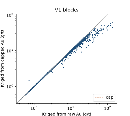
the capped grades feed the estimate as any other column. ordinary kriging estimates 5 m blocks inside the V1 solid from the raw and from the capped composites of V1, with one variogram and search. the extreme channels no longer spread their grade over their neighborhood: the richest blocks drop below the diagonal and the low-grade ones stay on it. the blocks lose 5 % of their mean grade, against 11 % for the declustered composites, because most blocks draw on samples below the cap, which capping leaves unchanged.
v1 = quartz.filter(quartz["VEIN"] == "V1")
v1 = v1.with_column("AU_CAPPED", capping.transform("AU_GPT", domain_column="VEIN", data=v1))
blocks = bt.BlockModel.from_extents(data["vein_V1"], size=(5.0, 5.0, 5.0))
targets = blocks.coords[data["vein_V1"].contains(blocks.coords)]
model = bt.experimental_variogram(v1, "AU_CAPPED", 10.0, 150.0).fit("spherical")
search = bt.Search(80.0, max_samples=24)
kriged = {
    column: bt.OrdinaryKriging(model, search).fit(v1, column).predict(targets)
    for column in ("AU_GPT", "AU_CAPPED")
}
for column, grades in kriged.items():
    print(f"{column}: {np.isfinite(grades).sum()} blocks, mean {np.nanmean(grades):.2f} g/t")
print(
    f"composites: {v1['AU_GPT'] @ v1['w'] / v1['w'].sum():.2f} and {v1['AU_CAPPED'] @ v1['w'] / v1['w'].sum():.2f} g/t"
)
Out:
AU_GPT: 5225 blocks, mean 7.73 g/t
AU_CAPPED: 5225 blocks, mean 7.31 g/t
composites: 8.52 and 7.60 g/t
fig, ax = plt.subplots(figsize=(4.5, 4))
ax.scatter(kriged["AU_GPT"], kriged["AU_CAPPED"], s=2, color=ACCENT)
ax.axline((0, 0), slope=1, color=GRAY, lw=0.8)
ax.axhline(capping.caps_["V1"], color=HIGHLIGHT, ls="--", lw=0.8, label="cap")
ax.set(xscale="log", yscale="log", xlabel="Kriged from raw Au (g/t)", ylabel="Kriged from capped Au (g/t)")
ax.set_title("V1 blocks")
ax.legend(loc="lower right")
save(fig, "kriged")
in a pipeline
Capping has fit, transform and fit_transform like NormalScore, so the two chain: cap, then score, the usual
preparation for a gaussian simulation. fitted once, both apply to new samples: a 500 g/t sample is capped to 81 g/t
before scoring, so its score is that of the cap. the fitted caps round-trip through JSON and pickle.
pipeline = bt.Capping(quantile=0.99)
capped = pipeline.fit_transform("AU_GPT", domain_column="VEIN", weights="w", data=v1)
scores = bt.NormalScore().fit(capped, weights=v1["w"])
new = np.array([0.5, 5.0, 50.0, 500.0])
print(scores.transform(pipeline.transform(new, domains=["V1"] * 4)).round(3))
restored = bt.Capping.from_json(pipeline.to_json())
print(restored.caps_ == pipeline.caps_)
Out:
[-1.305  0.386  1.981  2.658]
True
Total running time of the script: ( 0 minutes 0.692 seconds)
Download Python source code: example_04_03.py