Note
Click here to download the full example code
several training images
if the geology changes across a model, one image cannot hold all its patterns. SNESIM takes a training image per
domain, {domain: (model, column)}, and simulate picks each cell's image from its domain. the images share one set
of codes, so a code means the same in each domain.
import sys
from pathlib import Path

HERE = Path(__file__).parent if "__file__" in globals() else Path.cwd()
sys.path.insert(0, str(HERE.parents[1]))
import boitata as bt
import matplotlib.pyplot as plt
import numpy as np
from common import HIGHLIGHT, INK, save
from matplotlib.colors import ListedColormap

channels = bt.datasets.strebelle()
n = channels.count[0]
grid = bt.BlockModel((0, 0), (1, 1), (n, n))
objects build the second image: sand lenses about 36 by 10 cells, lying east-west, over 30 % of a grid the size of strebelle.
lens = {"shape": "ellipsoid", "code": 1, "proportion": 0.3, "radii": (18, 5), "azimuth": (80, 100)}
lenses = bt.object_training_image(grid, [lens], seed=4)
print(f"sand: channels {channels['facies'].mean():.1%}, lenses {lenses['facies'].mean():.1%}")
Out:
sand: channels 27.7%, lenses 30.2%
a line dipping east splits two domains: channels in the south, lenses in the north. twenty realizations, with the sand share of each domain against its image:
x, y = grid.x, grid.y
domains = np.where(y > 150 - 0.2 * x, "lenses", "channels")
snesim = bt.SNESIM({"channels": (channels, "facies"), "lenses": (lenses, "facies")})
summary = snesim.simulate(grid, n=20, seed=1, keep=[0], domains=domains)
for name, image in (("channels", channels), ("lenses", lenses)):
    share = summary.probabilities[domains == name, 1].mean()
    print(f"{name}: realizations {share:.1%} sand, image {image['facies'].mean():.1%}")
Out:
channels: realizations 29.2% sand, image 27.7%
lenses: realizations 30.4% sand, image 30.2%
codes = ListedColormap(["white", "black"])
boundary = grid.grid(domains == "lenses")[0]
fig, axes = plt.subplots(1, 4, figsize=(15, 4), layout="constrained")
panels = (
    (channels["facies"], "Image: channels", codes),
    (lenses["facies"], "Image: lenses", codes),
    (summary.realizations[0], "Realization 1", codes),
    (summary.probabilities[:, 1], "P(sand), 20 realizations", "gray_r"),
)
for ax, (values, title, cmap) in zip(axes, panels):
    im = ax.imshow(grid.grid(values)[0], origin="lower", cmap=cmap, vmin=0, vmax=1, interpolation="nearest")
    ax.set(title=title, xticks=[], yticks=[])
    for side in ax.spines.values():
        side.set(visible=True, color=INK, lw=0.6)
for ax in axes[2:]:
    ax.contour(boundary, levels=[0.5], colors=HIGHLIGHT, linewidths=1.2)
fig.colorbar(im, ax=axes[3], shrink=0.8, label="probability")
save(fig, "zones")
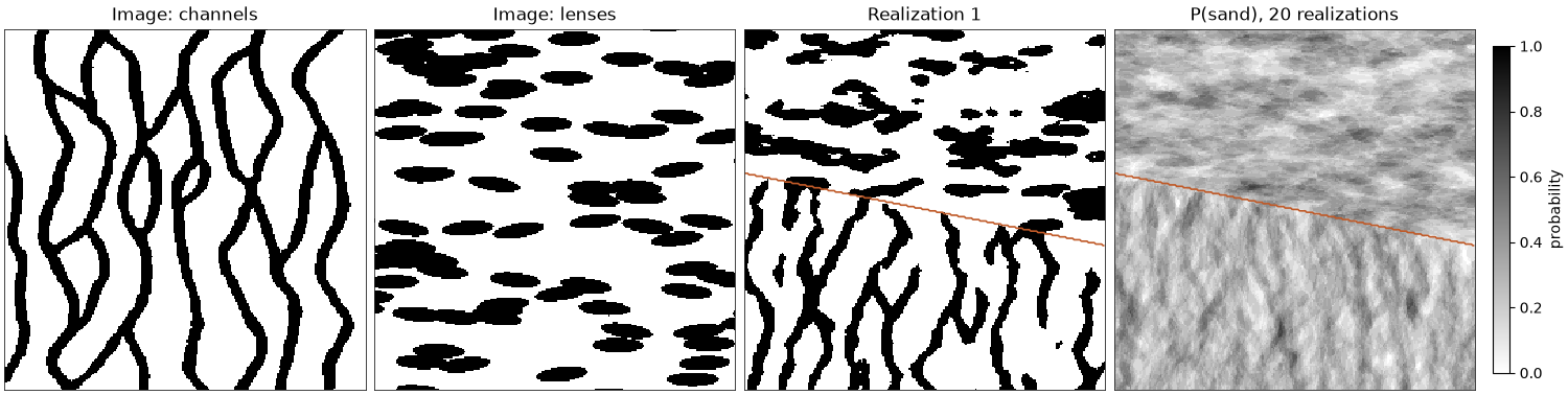
the boundary stays visible as a line. a cell next to it reads neighbors from both sides, which joins a channel to a
lens where they meet, but the change of pattern is abrupt. the images may differ in size and must share a kind: a
dict of continuous images works the same way, each domain drawing its values from its own image. hard data,
anisotropy and target_proportions combine with domains as without them.
Total running time of the script: ( 0 minutes 2.641 seconds)
Download Python source code: example_13_05.py