structural data¶

drill holes give contacts at a few places; mapping and oriented core give the orientation of the surface at many more. a synthetic fold shows what plane and lineation readings add to an implicit model, and how the field's gradient returns the dip.

import sys
from pathlib import Path

HERE = Path(__file__).parent if "__file__" in globals() else Path.cwd()
sys.path.insert(0, str(HERE.parents[1]))

import boitata as bt
import matplotlib.pyplot as plt
import numpy as np
from common import ACCENT, GRAY, HIGHLIGHT, INK, LIGHT, save

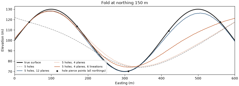
the fold, z = 100 + 30 sin(2πx / 400) with its axis north-south, is known without error. five holes pierce it, twelve outcrops along it give its dip and dip direction, and six other places give fold-axis lineations (plunge 0, trend 0). planes and lineations need the triharmonic kernel; one point above the surface sets which side is positive. isosurface extracts each modeled surface as a mesh, and Mesh.vertical_distance gives how far above it 400 points on the true surface lie: the elevation error over the whole fold.

rng = np.random.default_rng(4)


def surface(x):
    return 100 + 30 * np.sin(2 * np.pi * x / 400)


def true_dip(xy):
    slope = 30 * 2 * np.pi / 400 * np.cos(2 * np.pi * xy[:, 0] / 400)
    return np.degrees(np.arctan(np.abs(slope))), np.where(slope < 0, 90.0, 270.0)


def on_surface(xy):
    return np.c_[xy, surface(xy[:, 0])]


picks = on_surface(np.array([[40.0, 150], [170, 60], [310, 90], [420, 250], [560, 180]]))
outcrops = np.c_[np.linspace(20, 580, 12) + rng.uniform(-20, 20, 12), rng.uniform(0, 300, 12)]
planes = np.c_[on_surface(outcrops), np.column_stack(true_dip(outcrops))]
axis_readings = rng.uniform([0, 0], [600, 300], (6, 2))
lineations = np.c_[on_surface(axis_readings), np.zeros((6, 2))]
above = [[300.0, 150, 200]]
fits = {
    "5 holes": {},
    "5 holes, 12 planes": {"planes": planes},
    "5 holes, 4 planes": {"planes": planes[:4]},
    "5 holes, 4 planes, 6 lineations": {"planes": planes[:4], "lineations": lineations},
}
x = np.linspace(0, 600, 241)
z = np.linspace(0, 200, 801)
X, Z = np.meshgrid(x, z)
probe = rng.uniform([0, 0], [600, 300], (400, 2))
volume = bt.BlockModel(origin=(-5, -5, 0), size=(5, 5, 5), count=(122, 62, 40))
folds, depths = {}, {}
for name, readings in fits.items():
    folds[name] = bt.ImplicitModel(kernel="triharmonic").fit(above, [1.0], boundaries=picks, **readings)
    field = folds[name].predict(np.c_[X.ravel(), np.full(X.size, 150.0), Z.ravel()]).reshape(X.shape)
    depths[name] = z[np.argmin(np.abs(field), axis=0)]
    _, gradient = folds[name].predict(on_surface(probe), gradient=True)
    dip = np.degrees(np.arccos(np.abs(gradient[:, 2]) / np.linalg.norm(gradient, axis=1)))
    error = np.abs(folds[name].isosurface(volume).vertical_distance(on_surface(probe)))
    print(
        f"{name:>31}: surface within {np.median(error):4.1f} m (median), {error.max():4.1f} m (max); "
        f"dip within {np.median(np.abs(dip - true_dip(probe)[0])):3.1f}°"
    )

Out:

                        5 holes: surface within 13.6 m (median), 61.5 m (max); dip within 7.1°
             5 holes, 12 planes: surface within  1.9 m (median), 16.6 m (max); dip within 1.7°
              5 holes, 4 planes: surface within  7.1 m (median), 61.8 m (max); dip within 5.0°
5 holes, 4 planes, 6 lineations: surface within  5.3 m (median), 42.1 m (max); dip within 4.6°

twelve planes bring the surface from 14 m to 2 m of the truth (median) and the dip from 7° to under 2°. with four planes, the lineations add the direction of the fold axis and improve both.

fig, ax = plt.subplots(figsize=(10, 3.6), layout="constrained")
ax.plot(x, surface(x), color=INK, lw=2.2, label="true surface")
for (name, depth), color, style in zip(
    depths.items(), (GRAY, ACCENT, HIGHLIGHT, HIGHLIGHT), ("--", "-", ":", "-"), strict=True
):
    ax.plot(x, depth, color=color, ls=style, lw=1.2, label=name)
ax.scatter(picks[:, 0], picks[:, 2], color=INK, zorder=3, s=18, label="hole pierce points (all northings)")
ax.set(xlabel="Easting (m)", ylabel="Elevation (m)", title="Fold at northing 150 m", xlim=(0, 600))
ax.legend(ncol=2, loc="lower left", fontsize=8)
save(fig, "fold")

Fold at northing 150 m

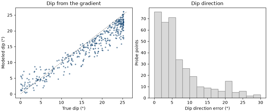
the gradient of the field is normal to the surface, so predict(..., gradient=True) returns the modeled dip and dip direction at any point, here against the truth at the 400 probe points of the twelve-plane model:

_, gradient = folds["5 holes, 12 planes"].predict(on_surface(probe), gradient=True)
dip = np.degrees(np.arccos(np.abs(gradient[:, 2]) / np.linalg.norm(gradient, axis=1)))
direction = np.degrees(np.arctan2(gradient[:, 0], gradient[:, 1])) % 360
truth_dip, truth_direction = true_dip(probe)
fig, (a, b) = plt.subplots(1, 2, figsize=(9, 3.8), layout="constrained")
bt.plot.scatter(truth_dip, dip, line=False, ax=a, color=ACCENT)
a.set(xlabel="True dip (°)", ylabel="Modeled dip (°)", title="Dip from the gradient")
b.hist(
    np.abs((direction - truth_direction + 180) % 360 - 180),
    bins=np.arange(0, 32, 2),
    color=LIGHT,
    edgecolor=GRAY,
)
b.set(xlabel="Dip direction error (°)", ylabel="Probe points", title="Dip direction")
save(fig, "dip")