variogram volume¶

a variogram map shows γ on one plane; in 3D the plane of best continuity is itself unknown. variogram_volume bins every pair by its lag vector into a cube of cells, the 3D variogram map, and reads the principal axes of continuity from a few hundred directions spread over the sphere. in each direction it finds the lag where γ reaches half the sill. under geometric anisotropy these lags trace an ellipsoid with the axes and ratios of the range ellipsoid, and its rotation and ratios go straight into Variogram. the axes here come from Zn composites across three stacked sulphide lenses, compared with the orientation of the lens solids.

import sys
from pathlib import Path

HERE = Path(__file__).parent if "__file__" in globals() else Path.cwd()
sys.path.insert(0, str(HERE.parents[1]))

import boitata as bt
import matplotlib.pyplot as plt
import numpy as np
from common import ACCENT, GRAY, HIGHLIGHT, save

composites and the lens orientation¶

Zn is high in the lenses and low in the rock around them, so the lenses are the continuous bodies. composites inside the lenses alone would say little about their orientation: a lens is a few meters thick, so every pair across it is a downhole pair. the example keeps all 2 m composites and takes Zn in logarithms to tame its skew. the orientation of each lens solid is the plane through its vertices, whose pole is the direction of least spread.

data = bt.datasets.stacked_sulphide_lenses()
holes = bt.Drillholes.from_tables(data)
composites = holes.composite(2.0, ["ZN_PCT"])
composites = composites.drop_null("ZN_PCT")
log_zn = np.log(composites["ZN_PCT"])
print(f"{len(composites)} composites")


def unit(azimuth, dip):
    az, dip = np.radians(azimuth), np.radians(dip)
    return np.array([np.cos(dip) * np.sin(az), np.cos(dip) * np.cos(az), -np.sin(dip)])


def plane(pole):
    """Dip and dip direction of the plane with this pole."""
    pole = pole if pole[2] > 0 else -pole
    return np.degrees(np.arccos(pole[2])), np.degrees(np.arctan2(pole[0], pole[1])) % 360


poles = []
for i in (1, 2, 3):
    vertices = data[f"lens_{i}"].coords
    pole = np.linalg.svd(vertices - vertices.mean(axis=0), full_matrices=False)[2][2]
    poles.append(pole if pole[2] > 0 else -pole)
    print(f"lens {i}: dips {plane(pole)[0]:.0f} degrees towards {plane(pole)[1]:03.0f}")
lens_pole = np.mean(poles, axis=0)
lens_pole /= np.linalg.norm(lens_pole)

Out:

13312 composites
lens 1: dips 59 degrees towards 111
lens 2: dips 61 degrees towards 110
lens 3: dips 59 degrees towards 110

the volume and its axes¶

lags of 15 m reach 225 m on each axis. each direction sums the pairs within 15 degrees of it; a wider cone averages in directions across the lenses and flattens the recovered dip.

volume = bt.variogram_volume(composites, log_zn, 15.0, 225.0, tolerance=15.0)
print("rotation (azimuth, dip, rake):", np.round(volume.rotation, 1))
print("ranges (major, semi, minor):  ", np.round(volume.ranges, 0))
print("ratios:                       ", np.round(volume.ratios, 2))
for name, (az, dip) in zip(("major", "semi-major", "minor"), volume.axes):
    print(f"{name:>10} axis: azimuth {az:05.1f}, dip {dip:4.1f}")

minor = unit(*volume.axes[2])
angle = np.degrees(np.arccos(abs(minor @ lens_pole)))
dip, direction = plane(minor)
lens_dip, lens_direction = plane(lens_pole)
print(f"plane of the major and semi-major axes: dips {dip:.0f} towards {direction:03.0f}")
print(f"mean lens plane:                        dips {lens_dip:.0f} towards {lens_direction:03.0f}")
print(f"minor axis to lens pole: {angle:.1f} degrees")

Out:

rotation (azimuth, dip, rake): [199.3  10.7 123.6]
ranges (major, semi, minor):   [179. 100.  80.]
ratios:                        [0.56 0.44]
     major axis: azimuth 199.3, dip 10.7
semi-major axis: azimuth 093.6, dip 54.9
     minor axis: azimuth 296.3, dip 32.9
plane of the major and semi-major axes: dips 57 towards 116
mean lens plane:                        dips 60 towards 110
minor axis to lens pole: 5.6 degrees

the major axis runs along strike, nearly horizontal; the semi-major axis runs down dip; the minor axis lies within a few degrees of the pole of the lenses. the plane of best continuity is the lens plane.

slices through the principal planes¶

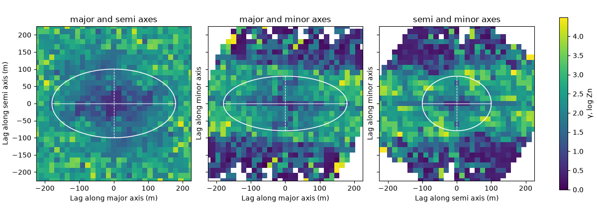
bt.plot.variogram_volume slices the cube through two principal axes and draws the range ellipse. in the plane of the lenses γ climbs slowly. across them it climbs fast, then drops where the lag reaches the next lens.

fig, axes = plt.subplots(1, 3, figsize=(12, 4.2), sharey=True, layout="constrained")
vmax = np.nanpercentile(volume.gammas, 98)
for ax, name in zip(axes, ("major-semi", "major-minor", "semi-minor")):
    bt.plot.variogram_volume(volume, plane=name, ax=ax, vmin=0, vmax=vmax)
    ax.set_title(name.replace("-", " and ") + " axes")
    ax.set_xlabel(ax.get_xlabel() + " (m)")
axes[0].set_ylabel(axes[0].get_ylabel() + " (m)")
fig.colorbar(axes[0].collections[0], ax=axes, label="γ, log Zn", shrink=0.85)
save(fig, "slices")

major and semi axes, major and minor axes, semi and minor axes

from the volume to a model¶

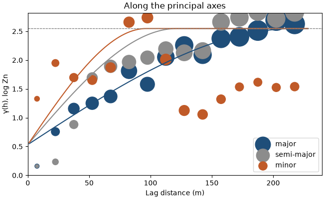
with the rotation and ratios held at the volume's values, experimental variograms along the three axes leave Variogram.fit_directional only the nugget, sill and range to find. across the lenses γ reaches the sill near 90 m and then falls back, as pairs 130 m apart land in the next lens: a hole effect the single structure ignores.

experimentals = [
    bt.experimental_variogram(composites, log_zn, 15.0, 225.0, azimuth=az, dip=dip, tolerance=15.0)
    for az, dip in volume.axes
]
model = bt.Variogram.fit_directional(
    experimentals, volume.axes, "spherical", rotation=volume.rotation, ratios=volume.ratios
)
structure = model.structures[0]
print(f"nugget {model.nugget:.2f}, sill {structure.sill:.2f}, major range {structure.range:.0f} m")

fig, ax = plt.subplots(figsize=(6.5, 4), layout="constrained")
for exp, direction, color, name in zip(
    experimentals, volume.axes, (ACCENT, GRAY, HIGHLIGHT), ("major", "semi-major", "minor")
):
    bt.plot.variogram(exp, variogram=model, direction=direction, ax=ax, color=color, label=name)
ax.legend(loc="lower right")
ax.set(xlabel="Lag distance (m)", ylabel="γ(h), log Zn", title="Along the principal axes")
save(fig, "axes")

Along the principal axes

Out:

nugget 0.53, sill 2.02, major range 218 m

Total running time of the script: ( 0 minutes 0.787 seconds)

Download Python source code: example_05_04.py

Download Jupyter notebook: example_05_04.ipynb

Gallery generated by mkdocs-gallery