Note
Click here to download the full example code
quick tour
one pass from samples to a checked estimate. walker lake has 470 samples of V (ppm) over a 260 × 300 m area, and
an exhaustive grid of 78 000 values over the same area to check the estimate against. each step fits in one cell and
links to the page that covers it in full.
import sys
from pathlib import Path

HERE = Path(__file__).parent if "__file__" in globals() else Path.cwd()
sys.path.insert(0, str(HERE.parents[1]))
import boitata as bt
import matplotlib.pyplot as plt
import numpy as np
from common import ACCENT, GRAY, INK, map_axes, save

samples = bt.datasets.walker_lake()
truth = bt.datasets.walker_lake_exhaustive()["V"].reshape(300, 260)
print(samples)
Out:
PointSet(470 points, crs: none)
  ID: Float64
  V: Float64
  U: Float64
  T: Float64
bt.datasets downloads a dataset once and caches it. the samples load as a PointSet: coordinates, plus one column
per variable. the exhaustive values wait for the checks at the end.
statistics
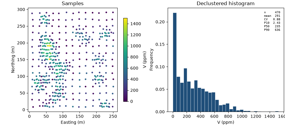
a first campaign sampled a 20 m grid and later ones infilled the rich zones, so the plain mean of the samples overstates the area. cell declustering weights each sample by the inverse of the sample count in its cell and keeps the cell size with the lowest mean (declustering).
declustering = bt.cell_declustering(samples, "V", sizes=np.arange(2.5, 102.5, 2.5))
weights = declustering.weights
naive, declustered = bt.describe(samples["V"]), bt.describe(samples["V"], weights=weights)
print(f"declustering cell {declustering.cell_size:.1f} m")
print(f"{'':12}{'mean':>6}{'CV':>6}{'P50':>6}{'P90':>6}{'max':>6}")
for name, stats in (
    ("naive", naive),
    ("declustered", declustered),
    ("exhaustive", bt.describe(truth.ravel())),
):
    print(
        f"{name:<12}{stats['mean']:>6.0f}{stats['cv']:>6.2f}{stats['P50']:>6.0f}{stats['P90']:>6.0f}"
        f"{stats['max']:>6.0f}"
    )

fig, (a, b) = plt.subplots(1, 2, figsize=(9.5, 4.2), layout="constrained")
points = a.scatter(*samples.coords[:, :2].T, c=samples["V"], s=8, vmin=0, vmax=1500)
map_axes(a, "Samples")
fig.colorbar(points, ax=a, shrink=0.8, label="V (ppm)")
bt.plot.histogram(samples["V"], weights=weights, bins=30, stats=True, ax=b, color=ACCENT)
b.set(title="Declustered histogram", xlabel="V (ppm)")
save(fig, "samples")
Out:
declustering cell 22.5 m
              mean    CV   P50   P90   max
naive          435  0.69   424   819  1528
declustered    291  0.88   235   636  1528
exhaustive     278  0.90   221   634  1631
declustering takes the mean from 435 to 291 ppm, 13 ppm above the exhaustive mean, and brings the median and P90 close to the true ones. the histogram is skewed to the right, with a peak of near-zero values and a thin tail up to 1528 ppm.
top cut
Capping clips the grades at a cap chosen from the data, here the declustered P99 (top cuts chooses a cap, and
capping transform compares the rules).
capping = bt.Capping(quantile=0.99).fit(samples["V"], weights=weights)
samples = samples.with_column("V_cut", capping.transform(samples["V"]))
print(
    f"cap {capping.caps_:.0f} ppm: {(samples['V'] > capping.caps_).sum()} samples cut, "
    f"{capping.metal_removed_:.1%} of the metal removed"
)
Out:
cap 982 ppm: 14 samples cut, 0.7% of the metal removed
the cap trims less than 1 % of the metal, since V has no erratic tail. the later steps use the capped column V_cut.
variogram
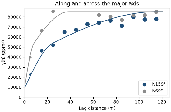
experimental_variogram computes γ(h) along one azimuth. Variogram.fit_directional fits one model (two
spherical structures with a nugget) to eight directions at once and finds the direction of greatest continuity
(experimental variograms, variogram fitting).
azimuths = np.arange(0, 180, 22.5)
directional = [bt.experimental_variogram(samples, "V_cut", 10.0, 120.0, azimuth=a) for a in azimuths]
model = bt.Variogram.fit_directional(
    directional, [(a, 0) for a in azimuths], ["spherical", "spherical"], weighting="count/gamma"
)
print(model)

major = model.rotation[0]
fig, ax = plt.subplots(figsize=(5.5, 3.6), layout="constrained")
for azimuth, color in ((major, ACCENT), (major + 90, GRAY)):
    experimental = bt.experimental_variogram(samples, "V_cut", 10.0, 120.0, azimuth=azimuth)
    bt.plot.variogram(
        experimental,
        variogram=model,
        direction=(azimuth, 0),
        ax=ax,
        color=color,
        label=f"N{azimuth % 180:.0f}°",
    )
ax.set(title="Along and across the major axis", xlabel="Lag distance (m)", ylabel="γ(h) (ppm²)")
ax.legend(loc="lower right")
save(fig, "variogram")
Out:
Variogram(nugget=8867.786210090486, structures=[Structure("spherical", sill=30452.04768457904, range=24.786734362667683), Structure("spherical", sill=45879.78702049813, range=115)], rotation=(159.196766259666, 0.0, 0.0), ratios=(0.3373516036246563, 1.0))
V is most continuous along N159°, with a range of 115 m. across it the range drops to about 40 m (a ratio of 0.34). the nugget holds a tenth of the sill.
kriging
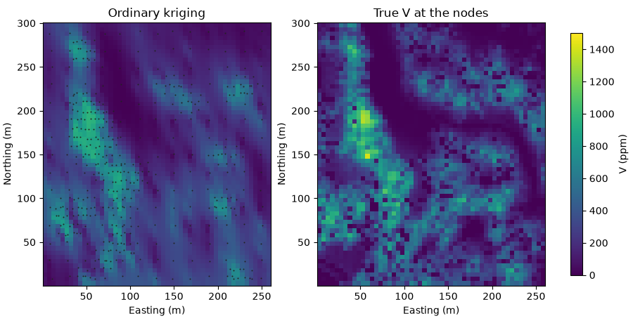
ordinary kriging estimates V on a 5 m grid from up to 24 samples in an ellipse aligned with the variogram. fit
takes the samples and the column, predict a BlockModel, and with_columns stores the results on the model
(ordinary kriging, search). the grid nodes fall on points of the exhaustive grid, so
the true value at each node joins the model as a second column.
grid = bt.BlockModel(origin=(3, 3), size=(5, 5), count=(52, 60))
search = bt.Search(radius=80, max_samples=24, min_samples=4, rotation=model.rotation, ratios=(0.5, 1.0))
kriging = bt.OrdinaryKriging(model, search).fit(samples, "V_cut")
nodes = grid.coords.astype(int)
grid = grid.with_columns(
    {"estimate": kriging.predict(grid), "truth": truth[nodes[:, 1] - 1, nodes[:, 0] - 1]}
)
print(grid)

extent = (0.5, 260.5, 0.5, 300.5)
fig, axes = plt.subplots(1, 2, figsize=(9, 4.6), layout="constrained")
for ax, name, title in ((axes[0], "estimate", "Ordinary kriging"), (axes[1], "truth", "True V at the nodes")):
    image = ax.imshow(grid.grid(name)[0], origin="lower", extent=extent, vmin=0, vmax=1500)
    map_axes(ax, title)
axes[0].scatter(*samples.coords[:, :2].T, s=2, color=INK, linewidths=0)
fig.colorbar(image, ax=axes, shrink=0.8, label="V (ppm)")
save(fig, "estimate")
Out:
BlockModel(regular, 3120 of 3120 cells, count [52, 60, 1], size [5.0, 5.0, 1.0], rotation [0.0, 0.0, 0.0])
  estimate: Float64
  truth: Float64
the estimate draws the NNW-trending rich zones of the truth, smoothed. kriging averages samples, so it misses the short-scale highs and lows.
checks
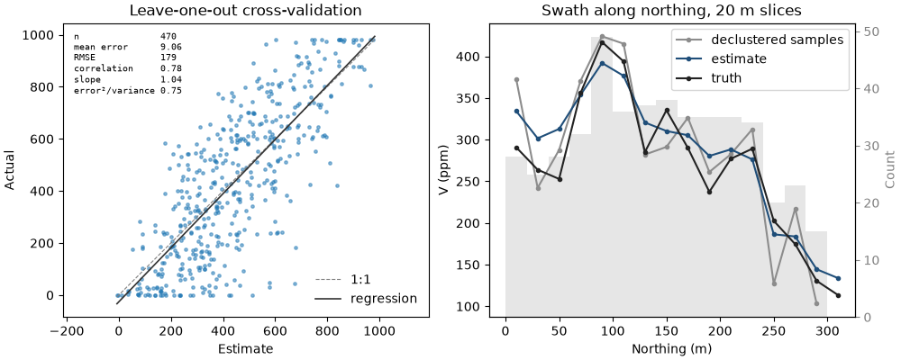
leave-one-out cross-validation re-estimates each sample from the others (cross-validation). a swath compares mean grades slice by slice for the declustered samples, the estimate and the truth (model checks, swaths).
cv = kriging.cross_validate()
print(f"cross-validation: RMSE {cv.rmse:.0f} ppm, correlation {cv.correlation:.2f}, slope {cv.slope:.2f}")
check = bt.compare("estimate", "truth", data=grid)
print(f"against the truth: RMSE {check['rmse']:.0f} ppm, correlation {check['correlation']:.2f}")
print(
    f"mean: estimate {grid['estimate'].mean():.0f}, declustered samples {declustered['mean']:.0f}, "
    f"truth {grid['truth'].mean():.0f} ppm"
)

fig, (a, b) = plt.subplots(1, 2, figsize=(10, 4), layout="constrained")
bt.plot.cross_validation(cv, ax=a)
a.set_title("Leave-one-out cross-validation")
series = [
    bt.swath(samples, "V_cut", 20.0, axis="y", weights=weights),
    bt.swath(grid, "estimate", 20.0, axis="y"),
    bt.swath(grid, "truth", 20.0, axis="y"),
]
bt.plot.swath(series, labels=["declustered samples", "estimate", "truth"], ax=b)
for line, color in zip(b.lines, (GRAY, ACCENT, INK), strict=True):
    line.set_color(color)
b.legend()
b.set(title="Swath along northing, 20 m slices", xlabel="Northing (m)", ylabel="V (ppm)")
save(fig, "checks")
Out:
cross-validation: RMSE 179 ppm, correlation 0.78, slope 1.04
against the truth: RMSE 154 ppm, correlation 0.79
mean: estimate 288, declustered samples 291, truth 277 ppm
the slope of 1.04 shows no conditional bias. cross-validation (RMSE 179 ppm) and the truth (RMSE 154 ppm) give errors of the same size. the estimate follows the swath of the truth and flattens its peaks. its mean matches the declustered samples and sits 4 % above the truth, a bias that no check against the samples can detect. storing containers in parquet saves a grid like this one to a file.
Total running time of the script: ( 0 minutes 0.798 seconds)
Download Python source code: example_01_01.py