Note
Click here to download the full example code
contacts
a nickel laterite logged down each hole as ferricrete (FERR), limonite (LIM), saprolite (SAP) and bedrock (BRK). should you estimate the horizons apart? grade against distance to a contact separates a hard boundary, where grade jumps, from a soft one, where grade changes gradually and samples on one side inform the other.
import sys
from pathlib import Path

HERE = Path(__file__).parent if "__file__" in globals() else Path.cwd()
sys.path.insert(0, str(HERE.parents[1]))
import boitata as bt
import matplotlib.pyplot as plt
from common import save

data = bt.datasets.nickel_laterite_profile()
assays = bt.merge_intervals(data["assays"], data["horizons"])
points = bt.Drillholes(data["collars"], data["surveys"], assays).samples()
print(f"{len(points)} assays of 1 m in {len(data['collars'])} holes")
Out:
10810 assays of 1 m in 448 holes
contact measures, down each hole, the distance from every sample of the two horizons to the nearest sample of the
other (negative inside) and bins them. plot.contact draws the mean per bin with the counts as light bars. the same
call runs on composites or on any points with hole ids and a domain column.
pairs = [("LIM", "SAP"), ("SAP", "BRK")]
tables = {
    (grade, inside): bt.contact(
        points,
        grade,
        domain_column="HORIZON",
        holes="HOLE_ID",
        inside=inside,
        outside=outside,
        max_distance=8.0,
        bin=1.0,
    )
    for grade in ["NI_PCT", "CO_PCT"]
    for inside, outside in pairs
}
for (grade, inside), table in tables.items():
    mean = dict(zip(table["distance"], table["mean"], strict=True))
    print(f"{grade} {inside} contact: {mean[-0.5]:.2f} % at -0.5 m, {mean[0.5]:.2f} % at +0.5 m")

fig, axes = plt.subplots(2, 2, figsize=(10, 6.4))
for ax, ((grade, inside), table) in zip(axes.flat, tables.items(), strict=True):
    outside = dict(pairs)[inside]
    bt.plot.contact(table, labels=(inside, outside), ax=ax)
    ax.set(title=f"{grade.split('_')[0].title()}, {inside} over {outside}", xlabel="Distance to contact (m)")
    ax.set_ylabel(f"Mean {grade.split('_')[0].title()} (%)")
fig.tight_layout()
save(fig, "contacts")
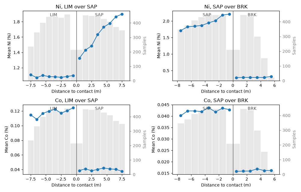
Out:
NI_PCT LIM contact: 1.10 % at -0.5 m, 1.32 % at +0.5 m
NI_PCT SAP contact: 2.21 % at -0.5 m, 0.29 % at +0.5 m
CO_PCT LIM contact: 0.12 % at -0.5 m, 0.04 % at +0.5 m
CO_PCT SAP contact: 0.04 % at -0.5 m, 0.02 % at +0.5 m
Ni is soft at the LIM/SAP contact: it rises from 1.10 to 1.32 % across it, then keeps climbing for several meters into the saprolite, so Ni in either horizon near the contact can borrow samples from the other. at the base of the saprolite it falls from 2.21 to 0.29 % within a meter, a hard boundary: keep bedrock samples out of the saprolite estimate. Co shows the other pattern, stepping from 0.12 to 0.04 % at the LIM/SAP contact and staying flat on each side. the same horizons can be a hard boundary for one grade and a soft one for another.
Total running time of the script: ( 0 minutes 1.622 seconds)
Download Python source code: example_03_07.py