Note
Click here to download the full example code
models larger than memory
a block model can stay in a parquet file and be processed a chunk at a time, so the disk limits its size instead of memory. here you simulate the iron ore of an iron formation plateau on millions of 5 m blocks, by domain and around a trend, without holding more than a million blocks at once.
import sys
from pathlib import Path

HERE = Path(__file__).parent if "__file__" in globals() else Path.cwd()
sys.path.insert(0, str(HERE.parents[1]))
import shutil
import tempfile
import time

import boitata as bt
import matplotlib.pyplot as plt
import numpy as np
from common import HIGHLIGHT, save
the dataset's block model codes each 25 × 25 × 12 m block with a lithology. two ore domains group them: hematite (friable, compact and canga) and itabirite (friable and compact). laterite and mafic dykes stay out. the 6 m composites take the domain of the block they fall in.
data = bt.datasets.iron_formation_plateau()
model = data["block_model"]
DOMAINS = {"HF": "hematite", "HC": "hematite", "CG": "hematite", "IF": "itabirite", "IC": "itabirite"}
coded = np.array([DOMAINS.get(c, "") for c in model["LITH"]], dtype=object)
model = model.with_columns({"domain": coded}).filter(coded != "")
coded = coded[coded != ""]

holes = bt.Drillholes.from_tables(data)
composites = holes.composite(6.0, ["FE_PCT"])
composites = composites.filter(model.contains(composites.coords)).drop_null("FE_PCT")
xyz, fe, hole = composites.coords, composites["FE_PCT"], composites["HOLE_ID"]
domain = model.sample(xyz, "domain")
for name in ("hematite", "itabirite"):
    inside = domain == name
    count = len(model.filter(model["domain"] == name))
    print(f"{name:10} {count:6,} blocks of 25 m, {inside.sum():5} composites")
Out:
hematite   14,889 blocks of 25 m,  1794 composites
itabirite  32,771 blocks of 25 m,  3635 composites
from_extents sizes a 5 m grid on the block model (block model from extents). the model keeps only the blocks whose
center falls in an ore block, found one level at a time. they form a masked model (the grid geometry plus the
sorted index of the cells present), written to parquet. BlockModelFile opens it without reading the blocks.
folder = Path(tempfile.mkdtemp())
grid = bt.BlockModel.from_extents(model, size=(5, 5, 5), snap=True)
nx, ny, nz = grid.count
plan = grid.coords[: nx * ny]
kept = [k * nx * ny + np.flatnonzero(model.contains(plan + (0, 0, 5 * k))) for k in range(nz)]
blocks = bt.BlockModel(grid.origin, grid.size, grid.count, index=np.concatenate(kept).astype(np.uint64))
bt.write_parquet(folder / "blocks.parquet", blocks)
file = bt.BlockModelFile(folder / "blocks.parquet")
size = (folder / "blocks.parquet").stat().st_size / 1e6
print(f"grid {grid.count}: {len(file):,} of {len(grid):,} blocks of 5 m kept, {size:.0f} MB")
Out:
grid [445, 405, 80]: 2,849,350 of 14,418,000 blocks of 5 m kept, 0 MB
weathering acts from the top of the plateau, so within a domain iron still drifts with position. a smooth trend per
domain (smooth trend), with a 400 m kernel flattened to 80 m vertically, takes that out, and you
simulate the residuals. the trend is smooth enough to evaluate on the 25 m blocks. map_blocks streams the file
through any function of a chunk and writes the columns it returns next to the input's: here each block's domain
and trend, looked up in the 25 m model.
at_data, at_model = np.zeros(len(fe)), np.zeros(len(model))
for name in ("hematite", "itabirite"):
    trend, _ = bt.detrend(xyz[domain == name], fe[domain == name], bandwidth=400.0, ratios=(1.0, 0.2))
    at_data[domain == name] = trend.predict(xyz[domain == name])
    at_model[coded == name] = trend.predict(model.coords[coded == name])
model = model.with_column("trend", at_model)


def attributes(chunk):
    return {"domain": model.sample(chunk.coords, "domain"), "trend": model.sample(chunk.coords, "trend")}


start = time.perf_counter()
bt.map_blocks(folder / "blocks.parquet", folder / "attributes.parquet", attributes)
print(f"domains and trend in {time.perf_counter() - start:.0f} s")
print(f"trend at the composites: variance {at_data.var():.0f} of {fe.var():.0f} %²")
Out:
domains and trend in 1 s
trend at the composites: variance 65 of 175 %²
turning bands simulates the bands of each realization once over the model's extent, then evaluates and
conditions them chunk by chunk. fitted with the domains and the trend at the data, each domain gets its own
normal-score transform of the residuals. simulate_to_parquet then reads each block's domain and trend from the
columns named by domain_column and trend. it writes the same summary simulate would return for the whole
model, plus the global statistics of each realization. keep= writes chosen realizations beside the summary, here
the first, as realization_0.
scores = bt.NormalScore().fit_transform(fe - at_data)
fitted = bt.experimental_variogram(xyz, scores, 15.0, 300.0).fit("spherical")
reach = fitted.structures[0].range
gaussian = fitted.standardized()
print(f"residual scores: nugget {gaussian.nugget:.2f}, range {reach:.0f} m")
bands = bt.TurningBands(gaussian, bands=100, search=bt.Search(radius=reach, max_samples=16))
bands.fit(xyz, fe, trend=at_data, domains=domain, holes=hole)

start = time.perf_counter()
result = bands.simulate_to_parquet(
    folder / "attributes.parquet",
    folder / "simulated.parquet",
    n=10,
    seed=1,
    cutoffs=[60.0],
    keep=[0],
    domain_column="domain",
    trend="trend",
)
seconds = time.perf_counter() - start
low, high = np.quantile(result["realization_above"][:, 0], [0.1, 0.9])
print(f"10 realizations in {seconds:.0f} s; blocks above 60 % Fe: P10 {low:.1%}, P90 {high:.1%}")
print(f"output {(folder / 'simulated.parquet').stat().st_size / 1e6:.0f} MB")
first = np.concatenate(
    [
        c["realization_0"]
        for c in bt.BlockModelFile(folder / "simulated.parquet").chunks(columns=["realization_0"])
    ]
)
print(f"first realization: mean {first.mean():.2f} % Fe, as accumulated {result['realization_mean'][0]:.2f}")
Out:
residual scores: nugget 0.36, range 35 m
10 realizations in 5 s; blocks above 60 % Fe: P10 22.3%, P90 22.6%
output 76 MB
first realization: mean 46.78 % Fe, as accumulated 46.78
mining selects 25 × 25 × 12 m blocks. with discretization, each block of a file is simulated at nodes, here
3 × 3 × 2, and the realizations are averaged over the block, as simulate(model.discretize(...), blocks=model)
would do. a node takes its block's domain and trend. the blocks load a chunk at a time, so their nodes stay within
memory too.
bt.write_parquet(folder / "model.parquet", model)
start = time.perf_counter()
panel = bands.simulate_to_parquet(
    folder / "model.parquet",
    folder / "model_simulated.parquet",
    n=10,
    seed=1,
    cutoffs=[60.0],
    domain_column="domain",
    trend="trend",
    discretization=(3, 3, 2),
)
seconds = time.perf_counter() - start
low, high = np.quantile(panel["realization_above"][:, 0], [0.1, 0.9])
print(f"{len(model):,} blocks of 25 m in {seconds:.0f} s; above 60 % Fe: P10 {low:.1%}, P90 {high:.1%}")
Out:
47,660 blocks of 25 m in 1 s; above 60 % Fe: P10 15.0%, P90 15.4%
averaging smooths the highs: about 15 % of the 25 m blocks pass 60 % Fe, against 22 % of the 5 m blocks.
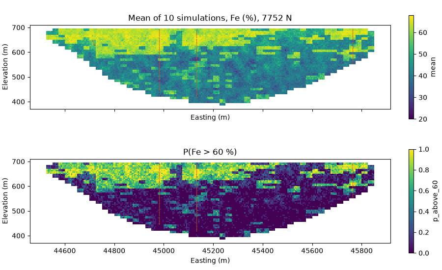
the output is too big for memory, so you collect the east-west section with the most composites from the chunks, reading only the columns it needs, into a small model of its own.
row = int(np.bincount(((xyz[:, 1] - grid.origin[1]) // 5).astype(int), minlength=ny).argmax())
columns = ["mean", "p_above_60"]
parts, index = {name: [] for name in columns}, []
for chunk in bt.BlockModelFile(folder / "simulated.parquet").chunks(columns=columns):
    on = (chunk.index // nx) % ny == row
    index.append(chunk.index[on])
    for name in columns:
        parts[name].append(chunk[name][on])
index = np.concatenate(index)
section = bt.BlockModel(
    (grid.origin[0], grid.origin[1] + 5 * row, grid.origin[2]),
    grid.size,
    (nx, 1, nz),
    index=index % nx + nx * (index // (nx * ny)),
    attributes={name: np.concatenate(parts[name]) for name in columns},
)
north = grid.origin[1] + 5 * (row + 0.5)
near = np.abs(xyz[:, 1] - north) < 5
fig, axes = plt.subplots(2, 1, figsize=(9, 5.5), layout="constrained", sharex=True)
bt.plot.section(section, "mean", axis="y", index=0, vmin=20, vmax=68, ax=axes[0])
bt.plot.section(section, "p_above_60", axis="y", index=0, vmin=0, vmax=1, ax=axes[1])
for ax, title in zip(axes, (f"Mean of 10 simulations, Fe (%), {north:.0f} N", "P(Fe > 60 %)"), strict=True):
    ax.scatter(xyz[near, 0], xyz[near, 2], s=2, color=HIGHLIGHT, linewidths=0)
    ax.set(title=title, xlabel="Easting (m)", ylabel="Elevation (m)")
save(fig, "section")
shutil.rmtree(folder, ignore_errors=True)
Total running time of the script: ( 0 minutes 18.577 seconds)
Download Python source code: example_02_10.py