Note
Click here to download the full example code
search
the search decides which samples inform each node. it has an ellipse along the continuity, octants against clustering,
passes that relax the search where the first finds too few samples, and a high-grade restriction on rich samples. the
example kriges walker lake V by ordinary kriging and checks it against the exhaustive values.
import sys
from pathlib import Path

HERE = Path(__file__).parent if "__file__" in globals() else Path.cwd()
sys.path.insert(0, str(HERE.parents[1]))
import boitata as bt
import matplotlib.pyplot as plt
import numpy as np
from common import ACCENT, GRAY, HIGHLIGHT, INK, LIGHT, map_axes, save
from matplotlib.colors import ListedColormap
from matplotlib.patches import Circle, Ellipse

samples = bt.datasets.walker_lake()
xy, v = samples.coords, samples["V"]
truth = bt.datasets.walker_lake_exhaustive()["V"].reshape(300, 260)
grid = bt.BlockModel(origin=(0.5, 0.5), size=(5, 5), count=(52, 60))
nodes = grid.coords.astype(int)
true_at_nodes = truth[nodes[:, 1] - 1, nodes[:, 0] - 1]

azimuths = np.arange(0, 180, 22.5)
directional = [bt.experimental_variogram(samples, "V", 10.0, 120.0, azimuth=a) for a in azimuths]
model = bt.Variogram.fit_directional(
    directional, [(a, 0) for a in azimuths], ["spherical", "spherical"], weighting="count/gamma"
)
kriging = bt.OrdinaryKriging(model, bt.Search(radius=80)).fit(samples, "V")


def rmse(estimate):
    return bt.compare(estimate, true_at_nodes)["rmse"]
ellipse and octants
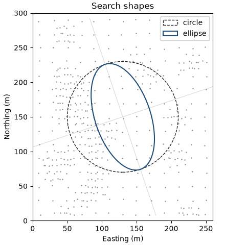
radius is the major semi-axis; rotation orients the ellipse like a variogram, and ratios shrink the other axes.
octant=True takes at most max_samples / 8 samples from each octant around the node, split along the axes of the
ellipse, so a dense cluster on one side cannot fill the neighborhood. with 2D data the sectors are the ellipse's four
quadrants, drawn below, with max_samples / 4 each. sectors=n splits the plane of the major and semi-major axes
into n equal angles instead, the first starting at the major axis, with max_per_sector samples each; it suits
thin tabular bodies, where the octants above and below the plane stay empty. with_search keeps the fitted samples
and the variogram and swaps the search.
ellipse = {"rotation": model.rotation, "ratios": (0.5, 1.0)}
searches = {
    "circle": bt.Search(radius=80, max_samples=24, min_samples=4),
    "ellipse": bt.Search(radius=80, max_samples=24, min_samples=4, **ellipse),
    "ellipse, octants": bt.Search(radius=80, max_samples=24, min_samples=4, octant=True, **ellipse),
    "ellipse, 6 sectors": bt.Search(
        radius=80, max_samples=24, min_samples=4, sectors=6, max_per_sector=4, **ellipse
    ),
}
print(f"{'search':>16}  RMSE  samples  mean distance  cross-validation RMSE")
for name, search in searches.items():
    estimator = kriging.with_search(search)
    d = estimator.predict(grid, diagnostics=True)
    print(
        f"{name:>16}  {rmse(d['value']):5.1f}  {np.nanmean(d['n_samples']):5.1f}  {np.nanmean(d['mean_distance']):9.1f} m"
        f"  {estimator.cross_validate().rmse:12.1f}"
    )

fig, ax = plt.subplots(figsize=(4.4, 4.8), layout="constrained")
ax.scatter(*xy[:, :2].T, s=3, color=GRAY, linewidths=0)
center = (130, 150)
azimuth = model.rotation[0]
ax.add_patch(Circle(center, 80, fill=False, color=INK, lw=1, ls="--", label="circle"))
ax.add_patch(Ellipse(center, 160, 80, angle=90 - azimuth, fill=False, color=ACCENT, lw=1.5, label="ellipse"))
for angle in (azimuth, azimuth + 90):
    dx, dy = 150 * np.sin(np.radians(angle)), 150 * np.cos(np.radians(angle))
    ax.plot([center[0] - dx, center[0] + dx], [center[1] - dy, center[1] + dy], color=LIGHT, lw=0.8, zorder=0)
ax.set(xlim=(0, 260), ylim=(0, 300))
map_axes(ax, "Search shapes")
ax.legend(loc="upper right", framealpha=0.9, frameon=True)
save(fig, "shapes")
Out:
          search  RMSE  samples  mean distance  cross-validation RMSE
          circle  154.8   21.4       31.0 m         185.5
         ellipse  155.1   23.5       29.5 m         185.4
ellipse, octants  154.8   20.7       29.5 m         185.1
ellipse, 6 sectors  154.5   19.4       27.7 m         184.3
the three searches give almost the same accuracy. the ellipse reaches closer samples along the continuity, and the quadrants keep about 21 of the 24 samples, fewer only where one side of a node is empty. kriging already gives far and redundant samples little weight, so the search matters more for speed, extrapolation and limiting negative weights than for the estimate at well-informed nodes.
passes
a list of searches runs as passes: nodes the first leaves unestimated go to the next, and diagnostics reports the
pass behind each. a first pass wanting eight samples within 30 m labels the nodes by how well they are informed, which
classification uses.
search = searches["ellipse, octants"]
passes = [bt.Search(radius=30, min_samples=8, max_samples=24, octant=True, **ellipse), search]
d = kriging.with_search(passes).predict(grid, diagnostics=True)
for p in (1, 2):
    s = d["pass"] == p
    error = bt.compare(d["value"][s], true_at_nodes[s])["rmse"]
    print(
        f"pass {p}: {s.mean():4.0%} of nodes, mean slope {np.mean(d['slope'][s]):.2f}, RMSE {error:.0f} ppm"
    )
print(f"RMSE of all nodes {rmse(d['value']):.1f} ppm")
Out:
pass 1:  40% of nodes, mean slope 0.97, RMSE 172 ppm
pass 2:  60% of nodes, mean slope 0.94, RMSE 143 ppm
RMSE of all nodes 155.1 ppm
pass-1 nodes have the higher slope of regression and also the larger errors. the walker lake drilling is densest where
V is high and variable, so the best-informed nodes are also the hardest ones.
high-grade restriction
high_grade=(800, 20) keeps samples above 800 ppm from informing nodes more than 20 m away.
print(f"{np.mean(v > 800):.0%} of the samples are above 800 ppm")
free = kriging.with_search(search)
capped = kriging.with_search(
    bt.Search(radius=80, max_samples=24, min_samples=4, octant=True, high_grade=(800, 20), **ellipse)
)
before, after = free.predict(grid), capped.predict(grid)
difference = after - before
error = before - true_at_nodes
for name, moved in (("lowered", difference < -5), ("raised", difference > 5)):
    print(
        f"{moved.sum()} nodes {name} by over 5 ppm; their mean error goes from {error[moved].mean():+.0f} ppm to "
        f"{(error + difference)[moved].mean():+.0f} ppm"
    )
print(
    f"cross-validation mean error {free.cross_validate().mean_error:+.1f} ppm without the restriction, "
    f"{capped.cross_validate().mean_error:+.1f} with"
)
Out:
12% of the samples are above 800 ppm
215 nodes lowered by over 5 ppm; their mean error goes from +11 ppm to +0 ppm
285 nodes raised by over 5 ppm; their mean error goes from -3 ppm to +8 ppm
cross-validation mean error +10.7 ppm without the restriction, +12.2 with
extent = (0.5, 260.5, 0.5, 300.5)
fig, (a, b) = plt.subplots(1, 2, figsize=(8.4, 4.4), layout="constrained")
a.imshow(
    grid.grid(d["pass"])[0],
    origin="lower",
    extent=extent,
    cmap=ListedColormap([ACCENT, LIGHT]),
    vmin=0.5,
    vmax=2.5,
)
a.scatter(*xy[:, :2].T, s=2, color=INK, linewidths=0)
map_axes(a, "Search pass")
a.legend(
    handles=[
        plt.Line2D([], [], marker="s", ls="", color=c, label=f"pass {p}")
        for p, c in ((1, ACCENT), (2, LIGHT))
    ],
    loc="upper right",
    framealpha=0.9,
    frameon=True,
)
im = b.imshow(grid.grid(difference)[0], origin="lower", extent=extent, cmap="PuOr_r", vmin=-40, vmax=40)
rich = v > 800
b.scatter(*xy[~rich, :2].T, s=2, color=GRAY, linewidths=0)
b.scatter(*xy[rich, :2].T, s=8, color=HIGHLIGHT, linewidths=0, label="V > 800 ppm")
map_axes(b, "Change from the high-grade restriction")
b.set_ylabel("")
b.legend(loc="upper right", framealpha=0.9, frameon=True)
fig.colorbar(im, ax=b, shrink=0.8, label="ppm")
save(fig, "passes")
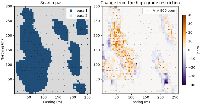
around isolated rich samples the restriction lowers the estimates where kriging overestimates most, and brings the mean error of those nodes to zero. inside the dense cluster of rich samples it raises them instead. there the rich samples 20 to 30 m away sit behind closer samples that screen them, so ordinary kriging gives them small negative weights, and dropping a negative weight on a high value raises the estimate. the restriction suits isolated high values; over all samples the cross-validation mean error changes little.
Total running time of the script: ( 0 minutes 0.438 seconds)
Download Python source code: example_06_06.py