Note
Click here to download the full example code
simulation at block support
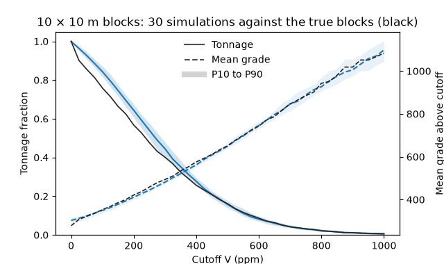
simulation reaches block support by averaging each realization on fine nodes over the nodes of each selective block, with no change-of-support model. the realizations give block grade-tonnage curves with their uncertainty and, pooled inside panels, localized block grades. the exhaustive walker lake grid gives the true 10 m blocks.
import sys
from pathlib import Path

HERE = Path(__file__).parent if "__file__" in globals() else Path.cwd()
sys.path.insert(0, str(HERE.parents[1]))
import boitata as bt
import matplotlib.pyplot as plt
import numpy as np
from common import ACCENT, GRAY, INK, save

samples = bt.datasets.walker_lake()
truth = bt.datasets.walker_lake_exhaustive()["V"].reshape(300, 260)
xy, v = samples.coords, samples["V"]
weights = bt.cell_declustering(samples, "V", sizes=np.arange(2.5, 102.5, 2.5)).weights
size = 10
SGS needs the variogram of normal scores with a unit sill: fitted along and across N170° (variogram fitting), then divided by its sill.
y = bt.NormalScore().fit(v, weights=weights).transform(v)
azimuths = (170, 260)
experimental = [bt.experimental_variogram(xy, y, 10, 120, azimuth=a) for a in azimuths]
fitted = bt.Variogram.fit_directional(experimental, [(a, 0) for a in azimuths], rotation=[170, 0, 0])
gaussian = fitted.standardized()
print(gaussian)
Out:
Variogram(nugget=0.3712292816104307, structures=[Structure("spherical", sill=0.6287707183895693, range=102.93174851181992)], rotation=(170.0, 0.0, 0.0), ratios=(0.34469006793164536, 1.0))
thirty realizations on 2.5 m nodes. blocks= averages each over the 16 nodes of each 10 × 10 m block before
summarizing, and grade_tonnage_cutoffs= accumulates each realization's block grade-tonnage curve as it runs, with
tonnes from density times block area here. grade_tonnage then reads the P10, P50 and P90 of the tonnage and the
mean grade above each cutoff, each quantity on its own.
cutoffs = np.linspace(0, 1000, 41)


def empirical(values):
    tonnage = np.array([(values >= c).mean() for c in cutoffs])
    grade = np.array([values[values >= c].mean() if (values >= c).any() else np.nan for c in cutoffs])
    return tonnage, grade


nodes = bt.BlockModel(origin=(0.5, 0.5), size=(2.5, 2.5), count=(104, 120))
blocks = bt.BlockModel(origin=(0.5, 0.5), size=(size, size), count=(26, 30))
sgs = bt.SGS(gaussian, bt.Search(radius=100, max_samples=24)).fit(xy, v, weights=weights)
summary = sgs.simulate(nodes, n=30, seed=7, blocks=blocks, grade_tonnage_cutoffs=list(cutoffs), density=1.0)
curves = summary.grade_tonnage(probabilities=[0.1, 0.5, 0.9])
true_block = empirical(truth.reshape(30, size, 26, size).mean(axis=(1, 3)).ravel())
share = curves["tonnage"] / curves["tonnage"][0]
for c in (300, 500, 800):
    k = np.searchsorted(cutoffs, c)
    p10, p90 = share[(curves["cutoff"] == cutoffs[k]) & np.isin(curves["probability"], [0.1, 0.9])]
    print(f"above {c} ppm: P10 {p10:.1%}, P90 {p90:.1%}, true {true_block[0][k]:.1%}")

fig, ax = bt.plot.grade_tonnage(curves, relative=True)
fig.set_size_inches(6.4, 3.8)
ax.plot(cutoffs, true_block[0], color=INK, lw=1.2)
fig.axes[-1].plot(cutoffs, true_block[1], color=INK, lw=1.2, ls="--")
ax.set(
    title=f"{size} × {size} m blocks: 30 simulations against the true blocks (black)", xlabel="Cutoff V (ppm)"
)
save(fig, "simulated-blocks")
Out:
above 300 ppm: P10 39.8%, P90 47.9%, true 40.1%
above 500 ppm: P10 14.1%, P90 17.7%, true 16.2%
above 800 ppm: P10 1.8%, P90 2.6%, true 2.1%
the band holds the true curve at each cutoff; at 300 ppm the truth sits at its lower edge.
a mine plan reads uncertainty over production volumes. groups= labels each block with its volume, here six 50 m
strips of northing standing for periods, and summarizes each realization's mean per period, one row per label.
window= gives each block the mean of the 50 × 50 m box centered on it, the boxes overlapping. both stream like
blocks= and feed the same summaries, here the relative error at 90 % confidence: half the P5–P95 interval over the
mean.
periods = blocks.y // 50
for label, volumes in (
    ("blocks", {}),
    ("periods", {"groups": periods}),
    ("50 m windows", {"window": (50, 50)}),
):
    error = sgs.simulate(
        nodes, n=30, seed=7, blocks=blocks, quantiles=[0.05, 0.95], **volumes
    ).relative_error()
    print(f"{label}: {len(error)} rows, median relative error {np.median(error):.1%}")
Out:
blocks: 780 rows, median relative error 58.8%
periods: 6 rows, median relative error 11.0%
50 m windows: 780 rows, median relative error 24.1%
the median error falls from 59 % on single blocks to 24 % on 50 m windows and 11 % on periods of 130 blocks.
tolerances= adds each row's precision, the share of realizations within ±15 % of its mean; a common criterion
for measured resources asks that share to reach 90 %. validate compares the summary with the true blocks. covered
marks a block whose true grade lies within the maximum expected error (MEE) of its mean, the relative error at 90 %
confidence, and cutoff= flags blocks classified as ore while waste in truth (type 1) and the reverse (type 2).
true_blocks = truth.reshape(30, size, 26, size).mean(axis=(1, 3)).ravel()
checked = sgs.simulate(
    nodes, n=30, seed=7, blocks=blocks, cutoffs=[500], quantiles=[0.05, 0.95], tolerances=[0.15]
)
table = checked.validate(true_blocks, cutoff=500)
print(f"precision at ±15 % reaching 90 %: {np.mean(checked.precision[:, 0] >= 0.9):.1%} of blocks")
print(f"truth within the MEE: {np.mean(table['covered']):.1%} of blocks")
print(f"at 500 ppm: type 1 {np.mean(table['type_1']):.1%}, type 2 {np.mean(table['type_2']):.1%} of blocks")
Out:
precision at ±15 % reaching 90 %: 0.8% of blocks
truth within the MEE: 80.5% of blocks
at 500 ppm: type 1 2.1%, type 2 5.3% of blocks
single 10 m blocks almost never meet ±15 % at 90 %. the truth lies within the MEE for 80 % of blocks, short of the nominal 90 %, and 7 % of blocks fall on the wrong side of 500 ppm.
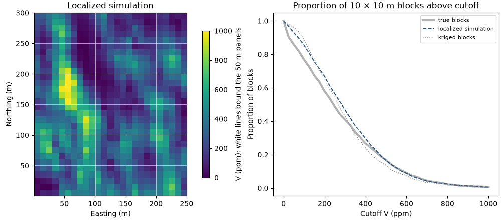
localization pools the realizations panel by panel. over the western 250 m, each 50 × 50 m panel holds 25 blocks. 25 blocks × 30 realizations give 750 values, sorted and cut into 25 chunks of 30, and the block ranked i by ordinary block kriging receives the mean of chunk i. the kriging uses the grade variogram, fitted like the one above.
grades = [bt.experimental_variogram(xy, v, 10, 120, azimuth=a) for a in azimuths]
grade = bt.Variogram.fit_directional(
    grades, [(a, 0) for a in azimuths], ["spherical", "spherical"], rotation=[170, 0, 0]
)
panels = bt.BlockModel(origin=(0.5, 0.5), size=(50, 50), count=(5, 6))
smus = panels.discretize(5)
search = bt.Search(radius=100, max_samples=24, min_samples=4)
kriged = bt.BlockKriging(grade, search, size=(size, size), discretization=(5, 5, 1)).fit(xy, v).predict(smus)
smus = smus.with_column("kriged", kriged)

west = bt.BlockModel(origin=(0.5, 0.5), size=(2.5, 2.5), count=(100, 120))
ensemble = sgs.simulate(west, n=30, seed=11, blocks=smus, keep=True)
localized = bt.localize(smus, "kriged", panels, ensemble.realizations)["localized"]
true_smu = truth[:, :250].reshape(30, size, 25, size).mean(axis=(1, 3))
for label, values in (("kriged", kriged), ("localized", localized)):
    r = bt.compare(values, true_smu.ravel())["correlation"]
    print(f"{label}: variance {values.var():.0f}, correlation with truth {r:.2f}")
print(f"true blocks: variance {true_smu.var():.0f}")
true_curve, kriged_curve, sim_curve = empirical(true_smu.ravel()), empirical(kriged), empirical(localized)

fig, (a, b) = plt.subplots(1, 2, figsize=(10, 4.4), layout="constrained", width_ratios=(1, 1.3))
extent = (0.5, 250.5, 0.5, 300.5)
image = a.imshow(np.reshape(localized, (30, 25)), origin="lower", extent=extent, vmin=0, vmax=1000)
a.vlines(np.arange(50.5, 250, 50), 0.5, 300.5, color="white", lw=0.6, alpha=0.7)
a.hlines(np.arange(50.5, 300, 50), 0.5, 250.5, color="white", lw=0.6, alpha=0.7)
a.set_aspect("equal")
a.set(title="Localized simulation", xlabel="Easting (m)", ylabel="Northing (m)")
fig.colorbar(image, ax=a, shrink=0.8, label="V (ppm); white lines bound the 50 m panels")
for (tonnage, _), color, style, label in (
    (true_curve, INK, {"lw": 3, "alpha": 0.35}, "true blocks"),
    (sim_curve, ACCENT, {"lw": 1.4, "ls": "--"}, "localized simulation"),
    (kriged_curve, GRAY, {"lw": 1.2, "ls": ":"}, "kriged blocks"),
):
    b.plot(cutoffs, tonnage, color=color, label=label, **style)
b.set(
    title=f"Proportion of {size} × {size} m blocks above cutoff",
    xlabel="Cutoff V (ppm)",
    ylabel="Proportion of blocks",
)
b.legend(fontsize=8)
save(fig, "localized-simulation")
Out:
kriged: variance 35064, correlation with truth 0.89
localized: variance 41003, correlation with truth 0.85
true blocks: variance 47350
each panel keeps the mean of its realizations, and its blocks the spread the simulation gives them: variance 41 411, between kriging's 35 064 and the true 47 350, with a correlation to the truth of 0.86 against kriging's 0.89. the pooling uses no change-of-support model, so its result depends on the realizations alone. uniform conditioning and MIK localization localize the same panels from a change-of-support model.
Total running time of the script: ( 0 minutes 0.576 seconds)
Download Python source code: example_08_03.py