saving and loading¶

models, transforms and searches save to JSON: to_json returns a string and the class's from_json builds the object back from it. a fitted transform keeps what it learned, so the loaded copy transforms new values the same way. containers and fitted estimators hold columns and go to parquet instead (storing containers in parquet).

import sys
from pathlib import Path

HERE = Path(__file__).parent if "__file__" in globals() else Path.cwd()
sys.path.insert(0, str(HERE.parents[1]))

import tempfile

import boitata as bt
import matplotlib.pyplot as plt
import numpy as np
from common import map_axes, save

a small workflow¶

walker lake V goes through five fitted pieces: cell declustering weights, a cap at the declustered P99, a normal-score transform, a variogram of the scores and a search. simple kriging of the scores, back-transformed, gives the estimate on a 5 m grid.

samples = bt.datasets.walker_lake()
declustering = bt.cell_declustering(samples, "V", sizes=np.arange(2.5, 102.5, 2.5))
capping = bt.Capping(quantile=0.99).fit("V", weights=declustering.weights, data=samples)
capped = capping.transform("V", data=samples)
normal_score = bt.NormalScore().fit(capped, weights=declustering.weights)
scores = normal_score.transform(capped)
variogram = bt.Variogram.fit(
    bt.experimental_variogram(samples, scores, 10.0, 120.0), ["spherical", "spherical"]
)
search = bt.Search(radius=60, max_samples=24, min_samples=4)

grid = bt.BlockModel(origin=(2.5, 2.5), size=(5, 5), count=(52, 60))
kriged = bt.SimpleKriging(variogram, search).fit(samples, scores).predict(grid)
estimate = normal_score.inverse_transform(kriged)
print(f"cap: {capping.caps_:.0f} ppm | declustered mean: {declustering.mean:.1f} ppm")
print(variogram)

Out:

cap: 982 ppm | declustered mean: 290.7 ppm
Variogram(nugget=0.3052597668357192, structures=[Structure("spherical", sill=0.501613916596432, range=39.9400880709822), Structure("spherical", sill=0.32454526508977327, range=63.403682315084254)], rotation=(0.0, 0.0, 0.0), ratios=(1.0, 1.0))

saving¶

each piece goes to its own file. the declustering file stores one weight per sample in the order of samples, and the normal-score file stores the fitted transform table. both grow with the data; the cap, the variogram and the search take a few hundred bytes.

folder = Path(tempfile.mkdtemp())
pieces = {
    "declustering": declustering,
    "capping": capping,
    "normal_score": normal_score,
    "variogram": variogram,
    "search": search,
}
for name, piece in pieces.items():
    (folder / f"{name}.json").write_text(piece.to_json())
    print(f"{name + '.json':>18}: {(folder / f'{name}.json').stat().st_size:>6} bytes")
print((folder / "search.json").read_text())

Out:

 declustering.json:   9959 bytes
      capping.json:    174 bytes
 normal_score.json:  21183 bytes
    variogram.json:    240 bytes
       search.json:    146 bytes
{"type":"Search","format":1,"min_samples":4,"max_samples":24,"radius":60.0,"max_per_hole":null,"octant":false,"anisotropy":null,"high_grade":null}

the files are plain JSON with a type and a format number. a reader of another type or a newer format raises InvalidInput instead of loading the wrong object.

loading and rerunning¶

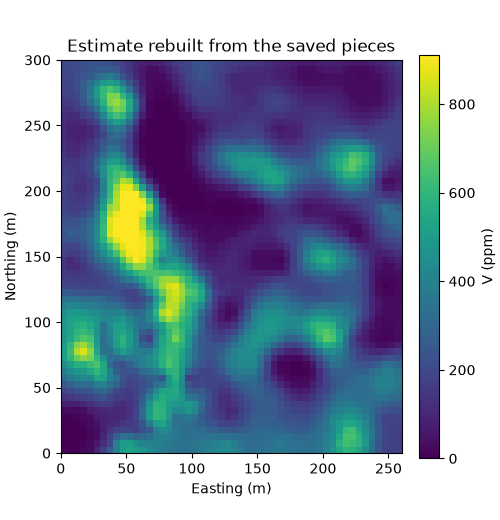
rerun sees only the folder and the samples. it reads the cap, the normal-score table, the variogram and the search, applies them in the same order and returns the estimate. it skips the weights, since the fitted cap and table already carry them. you load the weights separately for declustered statistics in a report.

def rerun(folder, samples):
    capping = bt.Capping.from_json((folder / "capping.json").read_text())
    normal_score = bt.NormalScore.from_json((folder / "normal_score.json").read_text())
    variogram = bt.Variogram.from_json((folder / "variogram.json").read_text())
    search = bt.Search.from_json((folder / "search.json").read_text())
    scores = normal_score.transform(capping.transform("V", data=samples))
    grid = bt.BlockModel(origin=(2.5, 2.5), size=(5, 5), count=(52, 60))
    kriged = bt.SimpleKriging(variogram, search).fit(samples, scores).predict(grid)
    return normal_score.inverse_transform(kriged)


again = rerun(folder, bt.datasets.walker_lake())
assert np.array_equal(again, estimate)
print("identical estimate:", np.array_equal(again, estimate))
weights = bt.Declustering.from_json((folder / "declustering.json").read_text()).weights
print(f"declustered mean from the saved weights: {np.average(capped, weights=weights):.1f} ppm (capped)")

fig, ax = plt.subplots(figsize=(5, 5.2), layout="constrained")
image = ax.imshow(
    grid.grid(again)[0], origin="lower", extent=(0, 260, 0, 300), vmin=0, vmax=np.quantile(again, 0.99)
)
fig.colorbar(image, ax=ax, shrink=0.8, label="V (ppm)")
map_axes(ax, "Estimate rebuilt from the saved pieces")
save(fig, "estimate")

Estimate rebuilt from the saved pieces

Out:

identical estimate: True
declustered mean from the saved weights: 288.8 ppm (capped)

the rerun matches bit for bit, because JSON writes each float with enough digits to read back the same number.

the same pair exists on Structure, Coregionalization, HighGrade, Categories, Trend and the other transforms (HermiteAnamorphosis, BoxCox, PPMT, PCA, MAF, StepwiseConditional, UniformConditioning, GaussianImputer, KernelDensity, GaussianMixture). these objects also pickle, through the same JSON. a fitted estimator such as the SimpleKriging above carries its samples, so it saves with to_parquet.

Total running time of the script: ( 0 minutes 0.231 seconds)

Download Python source code: example_01_03.py

Download Jupyter notebook: example_01_03.ipynb

Gallery generated by mkdocs-gallery