Note
Click here to download the full example code
spatial imputation
GaussianImputer (imputation) draws a missing value from the other
variables of the same sample. with spatial=, it also draws from nearby samples. the normal scores follow an
intrinsic model, in which every variable and every pair of variables share one correlogram scaled by the score
covariance. the imputer visits the samples along a random path and draws each missing score by simple cokriging from
its own row and from the nearest samples, those already imputed included. the variable here is density in the stacked
sulphide lenses, missing in 91% of all samples and in about half of the sulphide ones.
import sys
from pathlib import Path

HERE = Path(__file__).parent if "__file__" in globals() else Path.cwd()
sys.path.insert(0, str(HERE.parents[1]))
import boitata as bt
import matplotlib.pyplot as plt
import numpy as np
from common import HIGHLIGHT, INK, LIGHT, save

lenses = bt.datasets.stacked_sulphide_lenses()
intervals = bt.merge_intervals(lenses["assays"], lenses["lithology"])
samples = bt.Drillholes(lenses["collars"], lenses["surveys"], intervals).samples()
density = samples["DENSITY"]
sulphide = samples.filter(np.isin(samples["LITH"], ["MS", "SMS", "STR"])).drop_null("ZN_PCT")
columns = ["ZN_PCT", "PB_PCT", "CU_PCT", "AG_GPT", "AU_GPT", "DENSITY"]
data = np.column_stack([sulphide[c] for c in columns])
xyz, holes = sulphide.coords, sulphide["HOLE_ID"]
seen = ~np.isnan(data[:, 5])
print(f"density missing in {np.isnan(density).mean():.0%} of {len(density)} samples")
print(f"{len(data)} sulphide samples, density measured in {seen.sum()}")
Out:
density missing in 91% of 17848 samples
3358 sulphide samples, density measured in 1535
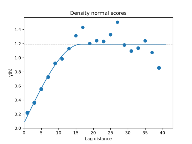
the spatial model is the variogram of the density normal scores, on 2 m lags: a small nugget and a range of about 16 m, shorter than the spacing between holes, so most of the information comes from the samples above and below in the same hole. the imputer rescales its sill to one.
scores = bt.NormalScore().fit_transform(data[seen, 5])
experimental = bt.experimental_variogram(xyz[seen], scores, 2.0, 40.0)
model = experimental.fit("spherical")
nugget, (structure,) = model.nugget, model.structures
print(f"nugget {nugget:.2f}, spherical sill {structure.sill:.2f}, range {structure.range:.1f} m")
fig, ax = bt.plot.variogram(experimental, variogram=model)
ax.set(title="Density normal scores")
save(fig, "variogram")
Out:
nugget 0.07, spherical sill 1.12, range 16.5 m
two checks hide measured densities and score the imputed ones against the truth: every other hole, as in imputation, and every other measured sample, which leaves the neighbors in the same hole. each imputer runs with 10 seeds, and both the error of one draw and that of the mean of the draws are root-mean-square.
order = np.flatnonzero(seen)
tests = {
    "every other hole": seen & np.isin(holes, np.unique(holes[seen])[::2]),
    "every other sample": np.isin(np.arange(len(data)), order[::2]),
}
imputers = {
    "same sample": lambda seed, holed: bt.GaussianImputer(seed=seed).fit(holed),
    "spatial": lambda seed, holed: bt.GaussianImputer(seed=seed, spatial=model).fit(holed, coords=xyz),
}
draws = {}
print(f"{'hidden':20}{'imputer':13}{'one draw':>9}{'mean':>7}{'sd':>6}")
for test, hidden in tests.items():
    holed = data.copy()
    holed[hidden, 5] = np.nan
    truth = data[hidden, 5]
    for name, make in imputers.items():
        d = np.array([make(seed, holed).transform(holed)[hidden, 5] for seed in range(10)])
        draws[test, name] = d
        one, mean = (bt.compare(x, truth)["rmse"] for x in (d[0], d.mean(axis=0)))
        print(f"{test:20}{name:13}{one:9.3f}{mean:7.3f}{d[0].std():6.2f}")
    print(f"{test:20}{'truth':13}{'':16}{truth.std():6.2f}")
Out:
hidden              imputer       one draw   mean    sd
every other hole    same sample      0.210  0.135  0.35
every other hole    spatial          0.216  0.138  0.35
every other hole    truth                          0.35
every other sample  same sample      0.220  0.135  0.36
every other sample  spatial          0.156  0.121  0.37
every other sample  truth                          0.36
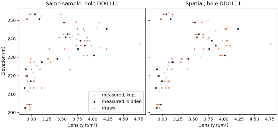
across holes the neighbors add almost nothing, since the hidden holes lie beyond the range of the variogram. within holes, one spatial draw errs by 0.16 t/m³ against 0.22 from the same sample alone, and both keep the spread of the truth. along one hole, the spatial draws follow the level of the measured densities around them.
hidden = tests["every other sample"]
counts = {h: (hidden & (holes == h)).sum() for h in np.unique(holes)}
hole = max(counts, key=counts.get)
rows = np.flatnonzero(holes == hole)
at = np.flatnonzero(hidden)
fig, axes = plt.subplots(1, 2, figsize=(9, 4.2), layout="constrained", sharey=True)
for ax, name in zip(axes, imputers):
    d = draws["every other sample", name]
    pick = np.isin(at, rows)
    kept = rows[~hidden[rows] & seen[rows]]
    ax.scatter(data[kept, 5], xyz[kept, 2], s=10, color=LIGHT, label="measured, kept")
    ax.scatter(data[at[pick], 5], xyz[at[pick], 2], s=10, color=INK, label="measured, hidden")
    for k in range(3):
        ax.scatter(
            d[k, pick], xyz[at[pick], 2], s=6, color=HIGHLIGHT, alpha=0.6, label="draws" if k == 0 else None
        )
    ax.set(xlabel="Density (t/m³)", title=f"{name.capitalize()}, hole {hole}")
axes[0].set_ylabel("Elevation (m)")
axes[0].legend(loc="lower right")
save(fig, "downhole")
the draws also keep the correlations. the normal-score correlation of density with Zn, Pb and Ag over the hidden samples, averaged over the draws, against the correlation fitted to the data:
hidden = tests["every other sample"]
holed = data.copy()
holed[hidden, 5] = np.nan
target = bt.GaussianImputer().fit(holed).correlation_[5]
ns = [bt.NormalScore().fit(data[:, j]) for j in (0, 1, 3)]
for name in imputers:
    d = draws["every other sample", name]
    z = [bt.NormalScore().fit(data[seen, 5]).transform(x) for x in d]
    r = [
        np.mean([np.corrcoef(n.transform(data[hidden, j]), zk)[0, 1] for zk in z])
        for n, j in zip(ns, (0, 1, 3))
    ]
    print(f"{name:12}" + "".join(f"{v:7.2f}" for v in r))
print(f"{'fitted':12}" + "".join(f"{target[j]:7.2f}" for j in (0, 1, 3)))
Out:
same sample    0.80   0.79   0.81
spatial        0.83   0.81   0.84
fitted         0.80   0.79   0.81
both stay within 0.03 of the fitted correlations. only the missing entries change, and the imputer returns measured
values as they are. transform takes coords= for new samples and otherwise reuses those given to fit. a
pure-nugget variogram gives the same draws as the non-spatial imputer, and MultivariateSimulation.fit(...,
impute=bt.GaussianImputer(spatial=model)) redraws the gaps this way in every realization
(multivariate simulation).
the intrinsic model is the simplest spatial model with the fitted correlations: one correlogram for all variables. here it comes from density, the variable being imputed, and grades with a different continuity borrow it too.
Total running time of the script: ( 0 minutes 6.773 seconds)
Download Python source code: example_04_07.py