Note
Click here to download the full example code
top cuts
gold in four quartz veins, V1 to V4, sampled by diamond holes and underground channels. a handful of extreme assays carry much of the metal, and one of them next to a block would lend it its grade. capping the grades at a top cut limits their influence. you need to decide where to cut and how much metal the cut costs.
import sys
from pathlib import Path

HERE = Path(__file__).parent if "__file__" in globals() else Path.cwd()
sys.path.insert(0, str(HERE.parents[1]))
import boitata as bt
import matplotlib.pyplot as plt
import numpy as np
from common import ACCENT, save

data = bt.datasets.vein_gold_grade_control()
intervals = bt.merge_intervals(data["assays"], data["lithology"])
holes = bt.Drillholes(data["collars"], data["surveys"], intervals)
composites = holes.composite(1.0, ["AU_GPT"], domain="LITH", categories=["VEIN"])
quartz = composites.filter(composites["LITH"] == "QV").drop_null("AU_GPT")
au = quartz["AU_GPT"]
print(f"{len(quartz)} composites of 1 m in quartz vein, mean Au {au.mean():.2f} g/t, max {au.max():.0f} g/t")
Out:
5826 composites of 1 m in quartz vein, mean Au 9.10 g/t, max 1192 g/t
channels crowd the developed levels, so the composites are first declustered in 20 m cells (declustering).
weights = bt.cell_declustering(quartz, "AU_GPT", cell_size=20.0).weights
print(f"declustered mean Au {np.average(au, weights=weights):.2f} g/t")
Out:
declustered mean Au 8.33 g/t
how much metal sits in the tail
capping tries caps at high quantiles and reports, for each, the share of weight above it, the metal removed, and the
capped mean and CV.
caps = bt.capping("AU_GPT", weights=weights, data=quartz)
print(f"{'cap':>7}{'above (%)':>11}{'metal (%)':>11}{'mean':>7}{'CV':>6}")
for cap, above, metal, mean, cv in zip(*(caps[c] for c in caps.column_names), strict=True):
    print(f"{cap:>7.1f}{100 * above:>11.2f}{100 * metal:>11.1f}{mean:>7.2f}{cv:>6.2f}")
Out:
    cap  above (%)  metal (%)   mean    CV
   18.1       9.99       36.5   5.29  1.07
   30.8       5.00       25.5   6.21  1.30
   49.2       2.50       17.6   6.86  1.51
   81.4       1.00       11.5   7.38  1.74
  120.3       0.44        8.1   7.66  1.92
  297.7       0.10        3.4   8.05  2.34
the top 1 % of the weight holds 11.5 % of the metal, and the top 10 % holds 36.5 %. the CV climbs from 1.07 at the lowest cap to 2.34 at the highest: the tail makes gold grades erratic.
the log-probability plot shows where the tail breaks away from the body of the distribution. the dotted tukey fences sit 1.5 interquartile ranges beyond the quartiles of log Au, and the dashed line is a cap at the declustered P99 of the vein.
stats = bt.describe_by("AU_GPT", "VEIN", weights=weights, quantiles=[0.5, 0.99], data=quartz)
top = dict(zip(stats["category"][:-1], stats["P99"][:-1], strict=True))
vein = quartz["VEIN"]
fig, axes = plt.subplots(1, 2, figsize=(9, 3.8), layout="constrained", sharey=True)
for ax, name in zip(axes, ["V1", "V2"], strict=True):
    keep = vein == name
    bt.plot.probability(
        au[keep], weights=weights[keep], log=True, cap=top[name], fences=1.5, ax=ax, color=ACCENT, ms=2
    )
    ax.set(title=f"{name}, declustered", xlabel="Au (g/t)")
    ax.legend(loc="lower right")
axes[1].set_ylabel("")
save(fig, "probability")
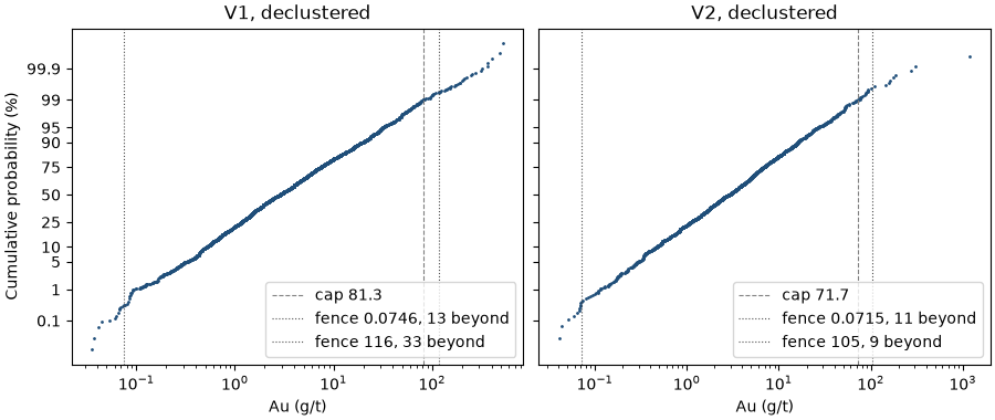
both veins plot near a straight line (a lognormal body) up to about P99. above it the points thin out, with the 1192 g/t channel alone at the top of V2. the upper fences, near 110 g/t, agree with a cap around P99.
one cap per vein
capping_report applies one cap per domain and compares the declustered statistics before and after, with the metal
removed; the last row pools the veins.
report = bt.capping_report("AU_GPT", top, domain_column="VEIN", weights=weights, data=quartz)
columns = ["domain", "cap", "n", "n_capped", "mean", "mean_capped", "cv", "cv_capped"]
print(
    f"{'vein':<5}{'cap':>7}{'n':>6}{'cut':>5}{'mean':>7}{'capped':>8}{'CV':>6}{'capped':>8}{'metal (%)':>11}"
)
for name, c, n, cut, mean, capped, cv, cv_capped in zip(*(report[k] for k in columns), strict=True):
    shown = "" if np.isnan(c) else f"{c:.1f}"
    print(
        f"{name:<5}{shown:>7}{n:>6.0f}{cut:>5.0f}{mean:>7.2f}{capped:>8.2f}{cv:>6.2f}{cv_capped:>8.2f}"
        f"{100 * (1 - capped / mean):>11.1f}"
    )
Out:
vein     cap     n  cut   mean  capped    CV  capped  metal (%)
V1      81.3  3659   47   8.52    7.60  2.60    1.72       10.8
V2      71.7  1968   23   7.95    6.73  4.31    1.67       15.4
V3      67.5    94    0   6.59    6.59  1.65    1.65        0.0
V4     183.5   105    1  15.06   14.96  2.04    2.01        0.7
all           5826   71   8.33    7.41  3.22    1.78       11.1
the caps cut 47 composites in V1 and 23 in V2, and remove 10.8 % and 15.4 % of their metal. pooled, the veins lose 11.1 % of the metal and the CV falls from 3.22 to 1.78. V3 and V4 hold about a hundred composites each, too few for a P99 to mean much: in V3 it is the maximum and cuts nothing. cap a small domain with the cap of a similar, larger one.
Total running time of the script: ( 0 minutes 0.615 seconds)
Download Python source code: example_03_05.py