Note
Click here to download the full example code
multiple indicator kriging
jura: 259 soil samples of heavy metals (mg/kg, coordinates in km) and 100 validation samples withheld from estimation. multiple indicator kriging (MIK) estimates the whole conditional distribution of Cd at each target.
import sys
from pathlib import Path

HERE = Path(__file__).parent if "__file__" in globals() else Path.cwd()
sys.path.insert(0, str(HERE.parents[1]))
import boitata as bt
import matplotlib.pyplot as plt
import numpy as np
from common import ACCENT, GRAY, HIGHLIGHT, INK, save

train = bt.datasets.jura()["prediction"]
test = bt.datasets.jura()["validation"]
xy, cd = train.coords, train["Cd"]
truth = test["Cd"]
limit = 0.8
lag, max_lag = 0.1, 1.5
search = bt.Search(radius=1.5, max_samples=24, min_samples=4)
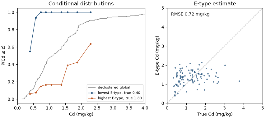
MIK kriges the indicators at the deciles of Cd and assembles the conditional distribution at each target. it corrects the kriged probabilities to rise from 0 to 1, and between thresholds the distribution follows the declustered data. one indicator variogram per threshold gives low and high values their own continuity; a single variogram at the median solves one system per target instead. ordinary kriging of Cd is the reference.
weights = bt.cell_declustering(xy, cd).weights
deciles = np.quantile(cd, np.linspace(0.1, 0.9, 9))
indicator_models = [
    bt.experimental_variogram(xy, (cd <= t).astype(float), lag, max_lag).fit("spherical") for t in deciles
]
summaries = {"cutoffs": [limit], "quantiles": [0.1, 0.5, 0.9]}
mik = bt.MultipleIndicatorKriging(indicator_models, search, deciles, tails=(0.0, cd.max()))
by_mik = mik.fit(xy, cd, weights=weights).predict(test, **summaries)
median = bt.MultipleIndicatorKriging(indicator_models[4], search, deciles, tails=(0.0, cd.max()))
by_median = median.fit(xy, cd, weights=weights).predict(test, **summaries)
ok = bt.OrdinaryKriging(bt.experimental_variogram(xy, cd, lag, max_lag).fit("spherical"), search).fit(
    train, "Cd"
)


def rmse(e):
    return bt.compare(e, truth)["rmse"]


exceeds = truth > limit
print(f"ordinary kriging: RMSE {rmse(ok.predict(test)):.3f} mg/kg")
for name, s in (("per-threshold variograms", by_mik), ("median indicator", by_median)):
    p = s.probability_above[:, 0]
    print(
        f"{name}: E-type RMSE {rmse(s.mean):.3f} mg/kg, mean P(Cd > {limit}) {p[exceeds].mean():.2f} where true"
        f" exceedance, {p[~exceeds].mean():.2f} elsewhere, mean correction {s.correction.mean():.3f}"
    )
inside = np.mean((truth >= by_mik.quantile_values[:, 0]) & (truth <= by_mik.quantile_values[:, 2]))
print(f"validation points inside their 10-90% interval: {inside:.0%}")
Out:
ordinary kriging: RMSE 0.777 mg/kg
per-threshold variograms: E-type RMSE 0.717 mg/kg, mean P(Cd > 0.8) 0.76 where true exceedance, 0.61 elsewhere, mean correction 0.060
median indicator: E-type RMSE 0.755 mg/kg, mean P(Cd > 0.8) 0.76 where true exceedance, 0.62 elsewhere, mean correction 0.005
validation points inside their 10-90% interval: 77%
the E-type estimate, the mean of each distribution, has a lower error than ordinary kriging, and the median-indicator shortcut gives most of that gain back. the distributions also carry the uncertainty: those at the lowest and highest validation estimates sit on either side of the declustered global one:
order = np.argsort(by_mik.mean)
fig, axes = plt.subplots(1, 2, figsize=(9, 3.8), layout="constrained")
sorted_cd = np.sort(cd)
cumulative = np.cumsum(weights[np.argsort(cd)]) / weights.sum()
axes[0].step(sorted_cd, cumulative, where="post", color=GRAY, lw=1, label="declustered global")
for i, color, label in ((order[0], ACCENT, "lowest E-type"), (order[-1], HIGHLIGHT, "highest E-type")):
    axes[0].plot(deciles, by_mik.cdf[i], "o-", color=color, ms=3, lw=1, label=f"{label}, true {truth[i]:.2f}")
axes[0].axvline(limit, color=INK, lw=0.6, ls=":")
axes[0].set(xlabel="Cd (mg/kg)", ylabel="P(Cd ≤ z)", title="Conditional distributions", xlim=(0, 4))
axes[0].legend(fontsize=8, loc="lower right")
axes[1].scatter(truth, by_mik.mean, s=12, color=ACCENT, alpha=0.7, linewidths=0)
axes[1].plot([0, 5], [0, 5], color=GRAY, ls="--", lw=1)
axes[1].set(
    xlim=(0, 5), ylim=(0, 5), xlabel="True Cd (mg/kg)", ylabel="E-type Cd (mg/kg)", title="E-type estimate"
)
axes[1].set_aspect("equal")
axes[1].text(0.2, 4.6, f"RMSE {rmse(by_mik.mean):.2f} mg/kg", color=INK)
save(fig, "distributions")
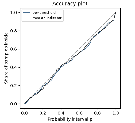
cross-validation re-estimates each sample's distribution from the others. besides the error of the E-type mean, it
scores the distributions with the brier score of each threshold's probability and with the accuracy plot, the share of
samples inside their own symmetric p-probability interval. points on or above the diagonal are accurate, and the
goodness statistic falls from 1 as the curve strays from it, twice as fast below. the diagnostics of predict count
the thresholds whose kriged probabilities broke the order relations at each target:
p = np.linspace(0, 1, 51)
fig, ax = plt.subplots(figsize=(4.4, 4), layout="constrained")
ax.plot([0, 1], [0, 1], color=GRAY, ls="--", lw=1)
for name, estimator, color in (("per-threshold", mik, ACCENT), ("median indicator", median, INK)):
    cv = estimator.cross_validate()
    print(
        f"{name}: E-type RMSE {cv.rmse:.3f} mg/kg, slope {cv.slope:.2f}, goodness {cv.goodness:.3f},"
        f" Brier {cv.brier.mean():.3f}"
    )
    ax.plot(p, cv.accuracy(p), color=color, lw=1.2, label=name)
diagnostics = mik.predict(test, diagnostics=True).diagnostics
violated = diagnostics["n_order_violations"] > 0
print(f"validation targets with order-relation violations: {violated.mean():.0%}")
ax.set(xlabel="Probability interval p", ylabel="Share of samples inside", title="Accuracy plot")
ax.set_aspect("equal")
ax.legend(fontsize=8, loc="upper left")
save(fig, "accuracy")
Out:
per-threshold: E-type RMSE 0.756 mg/kg, slope 1.06, goodness 0.939, Brier 0.131
median indicator: E-type RMSE 0.784 mg/kg, slope 0.97, goodness 0.944, Brier 0.133
validation targets with order-relation violations: 93%
at a panel centroid the distribution describes Cd at that one point. kriging the indicators over the panel instead,
with discretization=(4, 4, 1), gives the distribution of the point values within it, and localize takes the same
argument. each panel probability averages those of the points inside, so panels differ a little less and the order
relations need less correction. within 1 km the indicator variograms rise mostly at the nugget, which kriging at a
centroid already filters, so the two stay close here:
panels = bt.BlockModel(origin=(0.25, 0.0), size=(1.0, 1.0), count=(5, 6))
by_centroid = mik.predict(panels, cutoffs=[limit])
by_panel = mik.predict(panels, cutoffs=[limit], discretization=(4, 4, 1))
for name, s in (("centroids", by_centroid), ("1 km panels", by_panel)):
    print(
        f"{name}: std of P(Cd > {limit}) across panels {np.nanstd(s.probability_above[:, 0]):.3f},"
        f" mean correction {np.nanmean(s.correction):.4f}"
    )
shift = np.nanmean(np.abs(by_panel.probability_above[:, 0] - by_centroid.probability_above[:, 0]))
print(f"mean |panel - centroid| probability {shift:.3f}")
Out:
centroids: std of P(Cd > 0.8) across panels 0.188, mean correction 0.0218
1 km panels: std of P(Cd > 0.8) across panels 0.184, mean correction 0.0147
mean |panel - centroid| probability 0.016
Total running time of the script: ( 0 minutes 0.250 seconds)
Download Python source code: example_06_11.py