model checks¶

block kriging of walker lake V on 10 × 10 m blocks, checked against the declustered samples: the global bias, distributions side by side with validate_model, and swaths of grade and metal along easting and northing. the exhaustive grid gives the true blocks as a reference.

import sys
from pathlib import Path

HERE = Path(__file__).parent if "__file__" in globals() else Path.cwd()
sys.path.insert(0, str(HERE.parents[1]))

import boitata as bt
import matplotlib.pyplot as plt
import numpy as np
from common import ACCENT, GRAY, save

samples = bt.datasets.walker_lake()
truth = bt.datasets.walker_lake_exhaustive()["V"].reshape(300, 260)
xy, v = samples.coords, samples["V"]
azimuths = np.arange(0, 180, 22.5)
directional = [bt.experimental_variogram(xy, v, 10.0, 120.0, azimuth=a) for a in azimuths]
model = bt.Variogram.fit_directional(
    directional, [(a, 0) for a in azimuths], ["spherical", "spherical"], weighting="count/gamma"
)
weights = bt.cell_declustering(xy, v, sizes=np.arange(2.5, 102.5, 2.5)).weights

blocks = bt.BlockModel(origin=(0.5, 0.5), size=(10, 10), count=(26, 30))
search = bt.Search(radius=80, max_samples=24, min_samples=4, rotation=model.rotation, ratios=(0.5, 1.0))
kriging = bt.BlockKriging(model, search, size=(10, 10), discretization=(5, 5, 1)).fit(xy, v)
true_blocks = truth.reshape(30, 10, 26, 10).mean(axis=(1, 3)).ravel()
kriged = blocks.with_columns({"value": kriging.predict(blocks), "truth": true_blocks})

global bias¶

the mean of the blocks against the declustered mean of the samples. blocks of equal size weigh the same; for volumes or tonnages, pass them as weights.

bias = bt.global_bias(kriged["value"], v, data_weights=weights)
print(
    f"blocks {bias['estimate_mean']:.1f} ppm, declustered samples {bias['data_mean']:.1f} ppm, "
    f"bias {bias['relative']:+.1%}; true blocks {true_blocks.mean():.1f} ppm"
)

Out:

blocks 291.7 ppm, declustered samples 290.7 ppm, bias +0.3%; true blocks 278.0 ppm

distributions¶

validate_model sets the blocks against the samples, naive and declustered, with the true blocks as a reference. differences are relative to the declustered samples.

table = bt.validate_model(kriged, "value", samples, "V", weights=weights, reference="truth")
print(f"{'':12}{'n':>6}{'mean':>7}{'CV':>6}{'P10':>6}{'P50':>6}{'P90':>7}{'mean diff':>11}{'var. ratio':>11}")
for row in zip(
    *(table[c] for c in ["source", "n", "mean", "cv", "P10", "P50", "P90", "mean_diff", "variance_ratio"])
):
    source, n, mean, cv, p10, p50, p90, diff, ratio = row
    print(
        f"{source:<12}{n:>6.0f}{mean:>7.0f}{cv:>6.2f}{p10:>6.0f}{p50:>6.0f}{p90:>7.0f}{diff:>+11.1%}{ratio:>11.2f}"
    )

Out:

                 n   mean    CV   P10   P50    P90  mean diff var. ratio
naive          470    435  0.69    31   424    819     +49.8%       1.38
declustered    470    291  0.88     2   235    636      +0.0%       1.00
model          780    292  0.64    85   265    539      +0.3%       0.54
reference      780    278  0.78    26   239    576      -4.4%       0.72

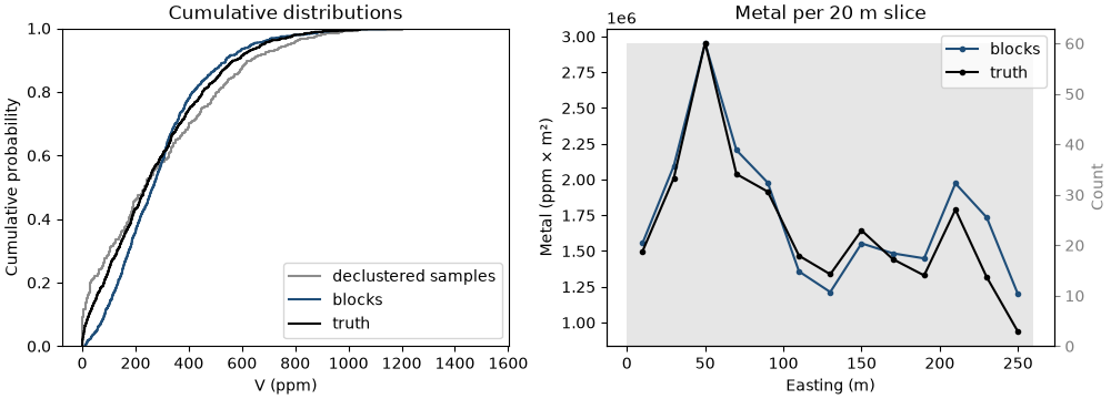
the blocks reproduce the declustered mean within 0.3 %. both sit about 5 % above the truth, a bias no check against the samples can see. the blocks are 10 × 10 m averages smoothed by kriging, so their variance is much smaller. the true blocks sit in between, since averaging over a block removes part of the sample variance. the cumulative distributions show the same smoothing: the blocks have fewer low and high grades than the true blocks, the declustered samples more. bt.plot.grade_tonnage draws the same comparison as tonnage and grade above cutoff (result plots). swaths of metal, grade × area per 20 m slice of easting, show where the estimate puts the metal; they add up to the metal of the whole model.

fig, axes = plt.subplots(1, 2, figsize=(10, 3.6), layout="constrained")
bt.plot.cdf([v, kriged["value"], true_blocks], weights=[weights, None, None], ax=axes[0])
metal = [bt.swath(kriged, g, 20.0, axis="x") for g in ("value", "truth")]
bt.plot.swath(metal, labels=["blocks", "truth"], y="metal", ax=axes[1])
for ax, colors in ((axes[0], (GRAY, ACCENT, "black")), (axes[1], (ACCENT, "black"))):
    for line, color in zip(ax.lines, colors, strict=True):
        line.set_color(color)
axes[0].legend(axes[0].lines, ["declustered samples", "blocks", "truth"])
axes[1].legend()
axes[0].set(xlabel="V (ppm)", title="Cumulative distributions")
axes[1].set(xlabel="Easting (m)", ylabel="Metal (ppm × m²)", title="Metal per 20 m slice")
save(fig, "distributions")

Cumulative distributions, Metal per 20 m slice

swaths¶

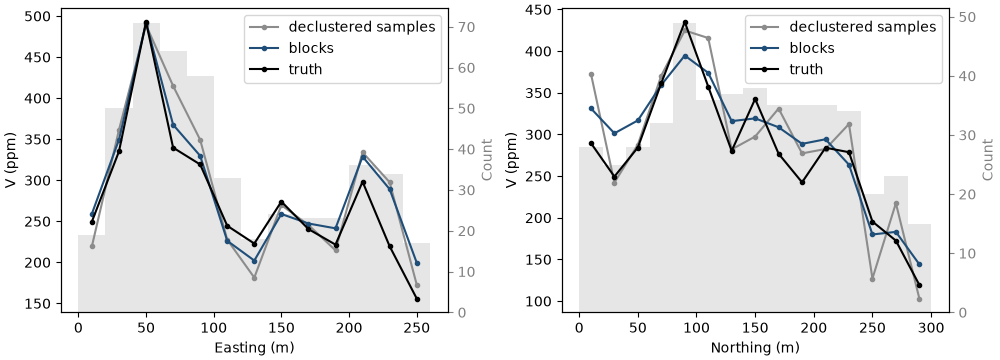
swaths reveal local bias: mean grade in 20 m slices along easting and northing, for the blocks, the declustered samples and the truth. the blocks track the truth slice by slice and are smoother than the samples, whose slice means scatter where few samples fall.

fig, axes = plt.subplots(1, 2, figsize=(10, 3.6), layout="constrained")
for ax, axis, name in ((axes[0], "x", "Easting (m)"), (axes[1], "y", "Northing (m)")):
    series = [
        bt.swath(samples, "V", 20.0, axis=axis, weights=weights),
        bt.swath(kriged, "value", 20.0, axis=axis),
        bt.swath(kriged, "truth", 20.0, axis=axis),
    ]
    bt.plot.swath(series, labels=["declustered samples", "blocks", "truth"], ax=ax)
    for line, color in zip(ax.lines, (GRAY, ACCENT, "black"), strict=True):
        line.set_color(color)
    ax.legend()
    ax.set(xlabel=name, ylabel="V (ppm)")
save(fig, "swaths")