Note

Click here to download the full example code

despiking

soil gold assays below the detection limit are all reported at 2 ppb, so four in ten samples share one value. a normal-score transform cannot split that spike, since the tied samples all get the same score. bt.despike breaks the ties by ranking each tied sample on the average rank of its neighbors within growing radii, with a seeded random draw as the last resort. values move by tiny offsets, so every untied sample keeps its rank.

import sys
from pathlib import Path

HERE = Path(__file__).parent if "__file__" in globals() else Path.cwd()
sys.path.insert(0, str(HERE.parents[1]))

import boitata as bt
import matplotlib.pyplot as plt
import numpy as np
from common import ACCENT, GRAY, HIGHLIGHT, LIGHT, map_axes, save

samples = bt.datasets.soil_geochemistry_survey()["samples"]
au = samples["AU_PPB"]
limit = au.min()
tied = au == limit
print(f"{tied.sum()} of {len(au)} samples at the detection limit ({limit:g} ppb)")

untied = bt.despike(samples, "AU_PPB", seed=0)
print(f"distinct values: {len(np.unique(au))} before, {len(np.unique(untied))} after")
print(f"largest change: {np.abs(untied - au).max():.1e} ppb")

ns = bt.NormalScore().fit(au)
spiked = ns.transform(au)
scores = bt.NormalScore().fit_transform(untied)

Out:

511 of 1227 samples at the detection limit (2 ppb)
distinct values: 174 before, 1227 after
largest change: 6.5e-05 ppb

without despiking, every sample at the limit takes the mean score of the tie. after despiking, the tied samples spread over the lower tail in the order of their neighborhoods:

z = np.linspace(-3.5, 3.5, 400)
bins = np.linspace(-3.5, 3.5, 36)
density = np.exp(-(z**2) / 2) / np.sqrt(2 * np.pi)
fig, axes = plt.subplots(1, 2, figsize=(9, 3.4), sharey=True, layout="constrained")
for ax, y, title in ((axes[0], spiked, "Tied: one spike"), (axes[1], scores, "Despiked: Gaussian")):
    ax.hist(y, bins, density=True, color=LIGHT, edgecolor=GRAY, lw=0.5)
    ax.hist(
        y[tied],
        bins,
        density=False,
        weights=np.full(tied.sum(), 1 / len(y) / np.diff(bins)[0]),
        color=HIGHLIGHT,
        alpha=0.6,
        label="at the detection limit",
    )
    ax.plot(z, density, color=ACCENT, lw=1.6, label="N(0, 1)")
    ax.set(title=title, xlabel="Normal score of Au")
axes[0].set_ylabel("Density")
axes[1].legend()
save(fig, "histograms")

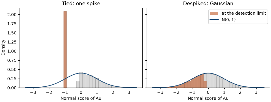
the ranking follows the neighborhoods: samples at the limit near high gold get the higher scores of the tie.

xyz = samples.coords
fig, ax = plt.subplots(figsize=(6.5, 4.6), layout="constrained")
ax.scatter(*xyz[~tied, :2].T, s=4, color=LIGHT)
points = ax.scatter(*xyz[tied, :2].T, c=scores[tied], s=9, cmap="cividis")
fig.colorbar(points, ax=ax, label="Normal score of tied samples", shrink=0.7)
map_axes(ax, "Samples at the detection limit, colored by despiked score")
save(fig, "map")

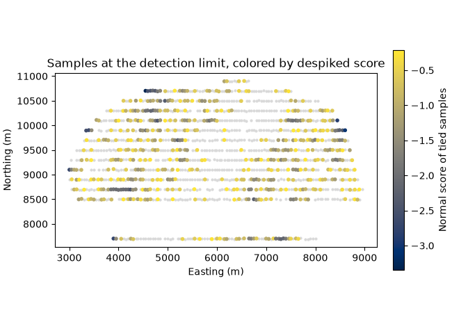
bt.despike(samples, ["AU_PPB", "AS_PPM"]) despikes several variables together, such as gold and arsenic, and orders samples tied in both the same way in each.

Total running time of the script: ( 0 minutes 0.353 seconds)

Download Python source code: example_03_06.py

Download Jupyter notebook: example_03_06.ipynb

Gallery generated by mkdocs-gallery