Note
Click here to download the full example code
smooth trend
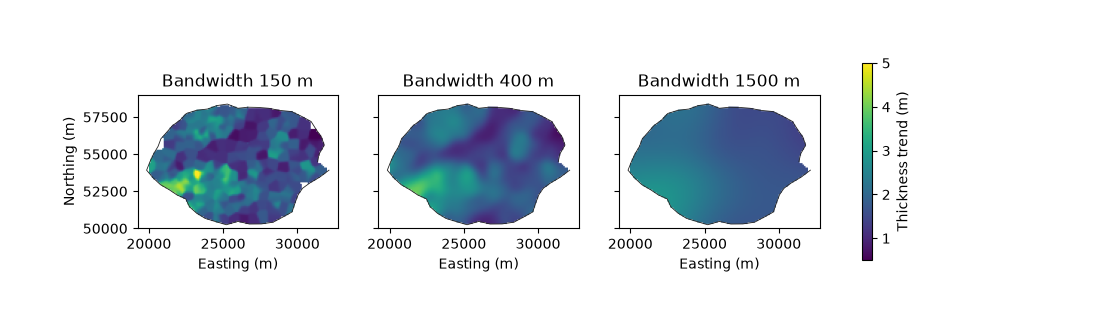
a moving-window trend: at each location, the declustered average of the boreholes under a gaussian kernel. maps of seam thickness for several bandwidths, the bandwidth chosen by leave-one-out error, the residuals, and the local proportions of the mining categories.
import sys
from pathlib import Path

HERE = Path(__file__).parent if "__file__" in globals() else Path.cwd()
sys.path.insert(0, str(HERE.parents[1]))
import boitata as bt
import matplotlib.pyplot as plt
import numpy as np
from common import ACCENT, GRAY, HIGHLIGHT, INK, map_axes, save
the coal seam was drilled on a regular mesh, then infilled where it is thick, so the boreholes over-represent thick coal. cell declustering weights correct that, and the trend averages the holes with these weights.
data = bt.datasets.coal_seam_thickness()
holes, grid, lease = data["boreholes"], data["grid"], data["boundary"]
weights = bt.cell_declustering(holes, "THICKNESS_M", cell_size=500.0).weights
thickness = holes["THICKNESS_M"]
print(
    f"{len(holes)} holes, mean {thickness.mean():.2f} m, declustered {np.average(thickness, weights=weights):.2f} m"
)

(x0, y0, _), (x1, y1, _) = grid.bounds
extent = (x0, x1, y0, y1)
outside = grid["INSIDE"] == 0


def image(ax, values, **kwargs):
    values = grid.grid(np.where(outside, np.nan, values))[0]
    shown = ax.imshow(values, origin="lower", extent=extent, **kwargs)
    ax.plot(*lease.coords[:, :2].T, color=INK, lw=0.6)
    return shown
Out:
295 holes, mean 2.23 m, declustered 1.98 m
bandwidth
detrend with a bandwidth fits a smooth trend instead of a polynomial. the bandwidth is the standard deviation of
the kernel: a small one follows every hole, a large one keeps only the regional shape. rotation and ratios, as for
a variogram, make the kernel anisotropic.
fig, axes = plt.subplots(1, 3, figsize=(11, 3.2), sharey=True)
norm = plt.Normalize(0.5, 5.0)
for ax, bandwidth in zip(axes, (150.0, 400.0, 1500.0)):
    trend, _ = bt.detrend(holes, "THICKNESS_M", bandwidth=bandwidth, weights=weights)
    shown = image(ax, trend.predict(grid), norm=norm)
    map_axes(ax, f"Bandwidth {bandwidth:.0f} m")
for ax in axes[1:]:
    ax.set_ylabel("")
fig.colorbar(shown, ax=axes, label="Thickness trend (m)", shrink=0.8)
save(fig, "bandwidths")
automatic choice
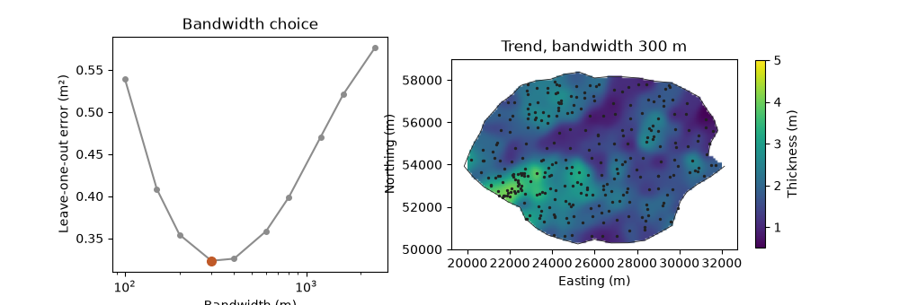
given several bandwidths, detrend keeps the one with the least leave-one-out error: it compares each hole with the
trend of the other holes and averages the squared differences with the declustering weights. too small a bandwidth
chases noise, and too large a one misses the shape. noisier data get a larger bandwidth.
candidates = [100, 150, 200, 300, 400, 600, 800, 1200, 1600, 2400]
trend, residuals = bt.detrend(holes, "THICKNESS_M", bandwidth=candidates, weights=weights)
print(f"chosen bandwidth {trend.bandwidth:.0f} m")

fig, (left, right) = plt.subplots(1, 2, figsize=(10, 3.4), gridspec_kw={"width_ratios": [1, 1.3]})
left.plot(trend.bandwidths, trend.scores, "o-", color=GRAY, ms=4)
best = trend.scores.argmin()
left.plot(trend.bandwidths[best], trend.scores[best], "o", color=HIGHLIGHT, ms=7)
left.set_xscale("log")
left.set_xlabel("Bandwidth (m)")
left.set_ylabel("Leave-one-out error (m²)")
left.set_title("Bandwidth choice")
shown = image(right, trend.predict(grid), norm=norm)
right.scatter(*holes.coords[:, :2].T, s=2, color=INK)
map_axes(right, f"Trend, bandwidth {trend.bandwidth:.0f} m")
fig.colorbar(shown, ax=right, label="Thickness (m)", shrink=0.8)
save(fig, "automatic")
Out:
chosen bandwidth 300 m
residuals
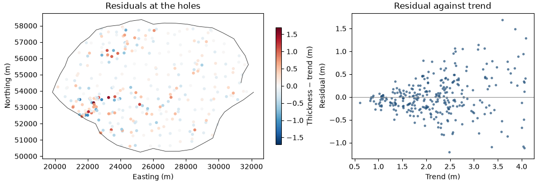
the residuals, thickness minus trend at the holes, keep the short-scale variation. they center on zero and correlate
weakly with the trend, but their spread grows with it: thick coal varies more, a proportional effect. normal-scoring
within classes of the trend, as SGS does with a trend, removes both.
at_holes = trend.predict(holes)
print(f"residual mean {np.average(residuals, weights=weights):+.3f} m, sd {residuals.std():.2f} m")
print(f"correlation with the trend {np.corrcoef(at_holes, residuals)[0, 1]:+.2f}")

fig, (left, right) = plt.subplots(
    1, 2, figsize=(10.5, 3.6), gridspec_kw={"width_ratios": [1.3, 1]}, layout="constrained"
)
left.plot(*lease.coords[:, :2].T, color=INK, lw=0.6)
limit = np.abs(residuals).max()
dots = left.scatter(*holes.coords[:, :2].T, c=residuals, s=10, cmap="RdBu_r", vmin=-limit, vmax=limit)
map_axes(left, "Residuals at the holes")
fig.colorbar(dots, ax=left, label="Thickness − trend (m)", shrink=0.8)
right.scatter(at_holes, residuals, s=6, color=ACCENT, alpha=0.6)
right.axhline(0, color=GRAY, lw=0.8)
right.set_xlabel("Trend (m)")
right.set_ylabel("Residual (m)")
right.set_title("Residual against trend")
save(fig, "residuals")
Out:
residual mean -0.011 m, sd 0.42 m
correlation with the trend +0.20
the trend at the holes and at the cells can feed a simulation
(SGS): SGS.fit(holes, "THICKNESS_M", trend=trend.predict(holes))
then simulate(grid, trend=trend.predict(grid)) simulates the thickness conditioned on the local trend. cells beyond
four bandwidths of every hole have no trend (NaN), so drop them first.
category proportions
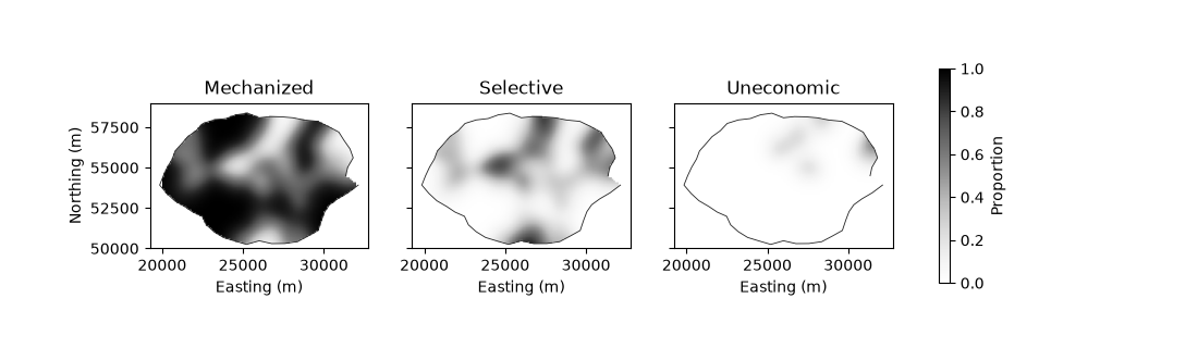
with categorical=True, detrend smooths the indicator of each category instead. the trend is then a table of local
proportions, one column per category, each in [0, 1] and summing to 1 at every cell.
categories, _ = bt.detrend(holes, "CATEGORY", bandwidth=candidates, weights=weights, categorical=True)
proportions = categories.predict(grid)
total = sum(proportions[name] for name in categories.categories)
print(
    f"bandwidth {categories.bandwidth:.0f} m; proportions sum to 1: {np.allclose(total[~np.isnan(total)], 1.0)}"
)

fig, axes = plt.subplots(1, 3, figsize=(11, 3.2), sharey=True)
for ax, name in zip(axes, categories.categories):
    shown = image(ax, proportions[name], vmin=0.0, vmax=1.0, cmap="Greys")
    map_axes(ax, name.capitalize())
for ax in axes[1:]:
    ax.set_ylabel("")
fig.colorbar(shown, ax=axes, label="Proportion", shrink=0.8)
save(fig, "proportions")
Out:
bandwidth 600 m; proportions sum to 1: True
Total running time of the script: ( 0 minutes 0.489 seconds)
Download Python source code: example_04_08.py