Note
Click here to download the full example code
censored normal-score transform
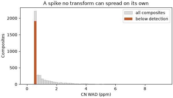
in the tailings reprocessing dataset, 46 % of the cyanide (WAD) samples are below the detection limit: those cells
hold the limit itself, flagged by CN_WAD_BDL. a plain normal-score transform sorts the data by value, so the ties at
the limit break in the order of the assay sheet. fit(..., censored=...) shuffles each such tie with a seed instead.
the below-detection scores then carry no order, and every other value, including ties at a different limit, keeps its
exact rank.
import sys
from pathlib import Path

HERE = Path(__file__).parent if "__file__" in globals() else Path.cwd()
sys.path.insert(0, str(HERE.parents[1]))
import boitata as bt
import matplotlib.pyplot as plt
import numpy as np
from common import ACCENT, GRAY, HIGHLIGHT, LIGHT, map_axes, save

assays = bt.datasets.tailings_reprocessing()["assays"]
assays = assays.drop_null("CN_WAD_PPM")
cn, bdl = assays["CN_WAD_PPM"], assays["CN_WAD_BDL"].astype(bool)
print(f"{len(cn)} composites; {bdl.mean():.0%} below the {cn[bdl][0]:g} ppm detection limit")

fig, ax = plt.subplots(figsize=(6, 3.4), layout="constrained")
bins = np.linspace(0, np.percentile(cn, 99), 60)
ax.hist(cn, bins=bins, color=LIGHT, edgecolor=GRAY, lw=0.4, label="all composites")
ax.hist(cn[bdl], bins=bins, color=HIGHLIGHT, label="below detection")
ax.set(xlabel="CN WAD (ppm)", ylabel="Composites", title="A spike no transform can spread on its own")
ax.legend()
save(fig, "histogram")
Out:
4129 composites; 46% below the 0.5 ppm detection limit
a tie broken by row order is still a tie
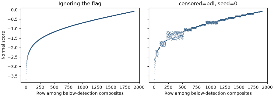
NormalScore().fit(cn) ignores the flag and sorts the below-detection composites by value. they are all equal, so the
stable sort leaves them in the order of the assay table. compare the score of each composite below detection with the
one before it in that table to see the artifact.
naive = bt.NormalScore().fit_transform(cn)


def rising_fraction(scores):
    tied = scores[bdl]
    return np.mean(tied[1:] > tied[:-1])


print(f"naive: {rising_fraction(naive):.0%} of consecutive below-detection rows have a rising score")
Out:
naive: 100% of consecutive below-detection rows have a rising score
almost every consecutive pair rises: the transform asserts that cyanide increases down the assay sheet within the
censored group, and the data say nothing about that. censored= shuffles the tie with a seed instead.
ns = bt.NormalScore()
aware = ns.fit_transform(cn, censored=bdl, seed=0)
print(
    f"censored=: {rising_fraction(aware):.0%} rising, a coin flip, as it should be for indistinguishable values"
)

fig, axes = plt.subplots(1, 2, figsize=(9, 3.2), sharey=True, layout="constrained")
row = np.arange(bdl.sum())
for ax, scores, title in ((axes[0], naive, "Ignoring the flag"), (axes[1], aware, "censored=bdl, seed=0")):
    ax.scatter(row, scores[bdl], s=3, color=ACCENT, alpha=0.5, linewidths=0)
    ax.set(xlabel="Row among below-detection composites", title=title)
axes[0].set_ylabel("Normal score")
save(fig, "ties")
Out:
censored=: 51% rising, a coin flip, as it should be for indistinguishable values
order is otherwise untouched
values above and below the limit, and ties at any other value, keep the ranks that NormalScore gives them without
censored. the scores of a censored fit back-transform to the reported data, limit values included, since the
transform invents nothing below the limit. inventing values there needs a reference distribution, which you cannot
combine with censored.
above = cn > cn[bdl][0]
print(
    f"lowest score above the limit exceeds every below-detection score: {aware[above].min() > aware[bdl].max()}"
)
back = ns.inverse_transform(aware)
print(f"round-trips to the reported data: {np.allclose(back, cn, atol=1e-6)}")
Out:
lowest score above the limit exceeds every below-detection score: True
round-trips to the reported data: True
composing with external drift kriging
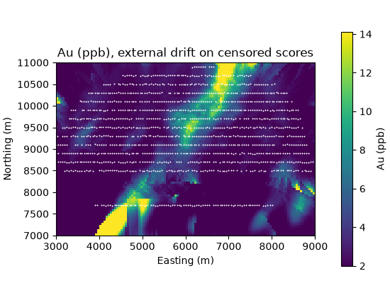
the soil geochemistry survey (external drift kriging) censors
gold and arsenic too. normal-score AU_PPB and AS_PPM with their own _BDL flags, then krige the gold score with
magnetics and elevation as external drift. the map below never reads an order into the samples at a detection limit.
soil = bt.datasets.soil_geochemistry_survey()
samples, covariates = soil["samples"], soil["covariates"]
samples = samples.with_columns(
    {c: covariates.sample(samples.coords[:, :2], c) for c in ("MAG_NT", "ELEVATION_M")}
)
au_bdl, as_bdl = samples["AU_BDL"].astype(bool), samples["AS_BDL"].astype(bool)
au_ns, as_ns = bt.NormalScore(), bt.NormalScore()
au_scores = au_ns.fit_transform(samples["AU_PPB"], censored=au_bdl, seed=0)
as_ns.fit_transform(samples["AS_PPM"], censored=as_bdl, seed=0)
print(
    f"AU_PPB {au_bdl.mean():.0%} censored, AS_PPM {as_bdl.mean():.0%} censored; both normal-scored the same way"
)

model = bt.experimental_variogram(samples.coords, au_scores, 200.0, 2500.0).fit(["spherical"])
search = bt.Search(radius=2500.0, max_samples=24, min_samples=4)
edk = (
    bt.ExternalDriftKriging(model, search, ["MAG_NT", "ELEVATION_M"])
    .fit(samples, au_scores)
    .predict(covariates)
)
grade = au_ns.inverse_transform(np.nan_to_num(edk))
grade[np.isnan(edk)] = np.nan
inside = covariates["INSIDE"] == 1
print(f"kriged Au inside the survey: mean {np.nanmean(np.where(inside, grade, np.nan)):.1f} ppb")

(x0, y0, _), (x1, y1, _) = covariates.bounds
fig, ax = plt.subplots(figsize=(5.5, 4.2), layout="constrained")
im = ax.imshow(
    covariates.grid(grade)[0], origin="lower", extent=(x0, x1, y0, y1), vmax=np.nanpercentile(grade, 98)
)
ax.scatter(samples.x, samples.y, s=2, color="white", linewidths=0)
map_axes(ax, "Au (ppb), external drift on censored scores")
fig.colorbar(im, ax=ax, shrink=0.8, label="Au (ppb)")
save(fig, "map")
Out:
AU_PPB 40% censored, AS_PPM 25% censored; both normal-scored the same way
kriged Au inside the survey: mean 3.5 ppb
Total running time of the script: ( 0 minutes 0.444 seconds)
Download Python source code: example_04_02.py