domain change tables¶

two categorical models of the same blocks differ block by block: an old and a new domain model, the most likely category and a realization, or a model before and after cleanup. domain_change cross-tabulates them: the tonnage moving from each class of the first model to each class of the second and, given a grade, the metal and mean grade of every cell. rows sum to the first model's classes, columns to the second's, the diagonal holds what stays, and the metal adds up to the model's. bt.plot.domain_change draws the table as a matrix.

import sys
import warnings
from pathlib import Path

HERE = Path(__file__).parent if "__file__" in globals() else Path.cwd()
sys.path.insert(0, str(HERE.parents[1]))
warnings.filterwarnings("ignore", ".*locations hold several samples")

import boitata as bt
import matplotlib.pyplot as plt
import numpy as np
from common import save

two rock models¶

the section of domain cleanup across the stacked sulphide lenses: the most likely rock from categorical indicator kriging of the logged rock types on 10 m cells, and the same model after remove_small_units gives units under 5000 m³ to the rock around them. ordinary kriging estimates zinc and density on the same cells from the 5 m composites, ignoring the rock types.

data = bt.datasets.stacked_sulphide_lenses()
intervals = bt.merge_intervals(data["assays"], data["lithology"])
drillholes = bt.Drillholes(data["collars"], data["surveys"], intervals)
composites = drillholes.composite(5.0, ["ZN_PCT", "DENSITY"], categories=["LITH"])
scheme = bt.Categories(
    ["OB", "HWS", "VCL", "SUL", "FWV"],
    mapping={"MS": "SUL", "SMS": "SUL", "STR": "SUL"},
    other="DYK",
    colors=["#d9d9d9", "#a9bfd3", "#8c8c8c", "#c05a28", "#1f4e79", "#e0c080"],
)
weights = bt.cell_declustering(composites, scheme.encode(composites["LITH"]), cell_size=50.0).weights
layers = (23.0, 55.0, 0.0)
variograms = [
    bt.Variogram([("spherical", 0.9, 400.0)], nugget=0.1, rotation=(0.0, 0.0, 0.0), ratios=(1.0, 0.05)),
    bt.Variogram([("spherical", 0.9, 500.0)], nugget=0.1, rotation=layers, ratios=(0.8, 0.2)),
    bt.Variogram([("spherical", 0.85, 400.0)], nugget=0.15, rotation=layers, ratios=(0.8, 0.2)),
    bt.Variogram([("spherical", 0.8, 150.0)], nugget=0.2, rotation=layers, ratios=(0.8, 0.25)),
    bt.Variogram([("spherical", 0.9, 500.0)], nugget=0.1, rotation=layers, ratios=(0.8, 0.2)),
    bt.Variogram([("spherical", 0.7, 40.0)], nugget=0.3),
]
passes = [
    bt.Search(150.0, max_samples=24, max_per_hole=6, rotation=layers, ratios=(1.0, 0.4)),
    bt.Search(300.0, max_samples=24, rotation=layers, ratios=(1.0, 0.4)),
]
cik = bt.CategoricalIndicatorKriging(variograms, passes, scheme=scheme)
cik.fit(composites, "LITH", weights=weights, holes="HOLE_ID")

center = np.array([12350.0, 29900.0, 0.0])
across = np.array([np.sin(np.radians(113.0)), np.cos(np.radians(113.0)), 0.0])
along = np.array([np.sin(np.radians(23.0)), np.cos(np.radians(23.0)), 0.0])
origin = center - 600.0 * across - 5.0 * along + [0.0, 0.0, -400.0]
section = bt.BlockModel(origin, (10.0, 10.0, 10.0), (120, 1, 80), rotation=(23.0, 0.0, 0.0))
topography = data["topography"]
section = section.filter(section.z < topography.sample(section.coords[:, :2], "Z"))
section = section.with_columns({"rock": cik.predict(section).most_likely}).drop_null("rock")

grade = bt.Variogram([("spherical", 0.8, 200.0)], nugget=0.2, rotation=layers, ratios=(0.8, 0.2))
search = bt.Search(300.0, max_samples=24, max_per_hole=6, rotation=layers, ratios=(1.0, 0.4))
for column in ["ZN_PCT", "DENSITY"]:
    known = composites.drop_null(column)
    kriged = bt.OrdinaryKriging(grade, search).fit(known, column, holes="HOLE_ID").predict(section)
    section = section.with_columns({column: kriged})
section = section.drop_null("ZN_PCT", "DENSITY")
section = section.with_columns({"clean": bt.remove_small_units(section, "rock", min_volume=5000.0)})
print(f"{len(section)} cells; {np.sum(section['rock'] != section['clean'])} change rock")

Out:

5205 cells; 37 change rock

the table¶

with the block volumes as weights and the kriged density, tonnage is in tonnes; with the zinc grades each cell also holds its metal (tonnes × %) and mean_grade. the table has one row per pair of rocks, in the order of the scheme. the rows of a rock sum to its tonnage before the cleanup, its column to its tonnage after, and the metal to the metal of the model: the cleanup moves tonnes and metal between rocks and creates or loses none.

table = bt.domain_change("rock", "clean", density="DENSITY", grades="ZN_PCT", scheme=scheme, data=section)
k = len(scheme)
tonnes = table["tonnage"].reshape(k, k)
block = section.volumes * section["DENSITY"]
before = [block[section["rock"] == c].sum() for c in range(k)]
after = [block[section["clean"] == c].sum() for c in range(k)]
print(f"rows are the rocks before: {np.allclose(tonnes.sum(axis=1), before)}")
print(f"columns are the rocks after: {np.allclose(tonnes.sum(axis=0), after)}")
print(f"unchanged: {np.trace(tonnes) / tonnes.sum():.1%} of {tonnes.sum() / 1e6:.1f} Mt")
zinc = np.sum(block * section["ZN_PCT"]) / 100
print(f"zinc in the table {np.sum(table['metal']) / 100 / 1e3:.2f} kt, in the model {zinc / 1e3:.2f} kt")

moved = table.filter((table["from"] != table["to"]) & (table["tonnage"] > 0))
for a, b, t, g in zip(moved["from"], moved["to"], moved["tonnage"], moved["mean_grade"]):
    print(f"{a:>4} to {b:4} {t / 1e3:5.1f} kt at {g:.2f} % Zn")

Out:

rows are the rocks before: True
columns are the rocks after: True
unchanged: 99.3% of 16.7 Mt
zinc in the table 68.04 kt, in the model 68.04 kt
 HWS to VCL   20.3 kt at 0.06 % Zn
 VCL to HWS   26.4 kt at 0.19 % Zn
 VCL to SUL   10.3 kt at 1.79 % Zn
 SUL to VCL    6.2 kt at 1.25 % Zn
 SUL to FWV   12.8 kt at 0.31 % Zn
 FWV to VCL   43.2 kt at 0.09 % Zn

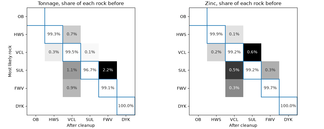
under 1 % of the tonnage changes rock, at grades far from random: the volcanic cells taken into the sulphides run near 1.8 % Zn, while the sulphide specks given to the footwall hold 0.3 %. the matrices show each row as shares of the rock it starts from, tonnage on the left and zinc on the right. the plot outlines the diagonal and leaves it blank, so the grays show only what moves.

fig, axes = plt.subplots(1, 2, figsize=(11, 4.4), layout="constrained")
for ax, value, title in zip(axes, ["tonnage", "metal"], ["Tonnage", "Zinc"]):
    bt.plot.domain_change(table, value=value, relative=True, fmt="{:.1%}", ax=ax)
    ax.set(title=f"{title}, share of each rock before", xlabel="After cleanup", ylabel="Most likely rock")
axes[1].set_ylabel("")
save(fig, "change")