Note
Click here to download the full example code
intrinsic coregionalization
an intrinsic coregionalization is the simplest multivariate variogram model: every direct and cross variogram has the
same normalized shape (one set of structures, ranges and anisotropy) scaled by one entry of a covariance matrix. the
correlation between two variables is then the same at every lag. Coregionalization.fit(..., intrinsic=True) fits the
shape to the pooled direct variograms, each divided by its sill, then fits the positive semi-definite covariance matrix.
Coregionalization.intrinsic builds one from a variogram and a matrix. either way the result is an ordinary
Coregionalization, so cokriging and cosimulation take it unchanged.
import sys
from pathlib import Path

HERE = Path(__file__).parent if "__file__" in globals() else Path.cwd()
sys.path.insert(0, str(HERE.parents[1]))
import boitata as bt
import matplotlib.pyplot as plt
import numpy as np
from common import ACCENT, GRAY, INK, save

jura = bt.datasets.jura()
train, test = jura["prediction"], jura["validation"]
xy = train.coords
cd, zn = train["Cd"], train["Zn"]
lag, max_lag = 0.1, 1.5
print(f"{len(cd)} samples, corr(Cd, Zn) {np.corrcoef(cd, zn)[0, 1]:.2f}")
Out:
259 samples, corr(Cd, Zn) 0.67
Cd and Zn
the data are the jura soil samples of coregionalization
(mg/kg, coordinates in km). experimental_variograms computes both variograms and the cross-variogram as a
VariogramSet, which the fit takes as it is. the intrinsic model has one shape (a nugget and two spherical
structures) and one 2 x 2 sill matrix.
experimentals = bt.experimental_variograms(train, ["Cd", "Zn"], lag, max_lag)
icm = bt.Coregionalization.fit(experimentals, ["spherical", "spherical"], intrinsic=True)
lmc = bt.Coregionalization.fit(experimentals, ["spherical", "spherical"])


def sill(model):
    return model.nugget + sum(s for _, _, s in model.structures)


for name, model in [("intrinsic", icm), ("full LMC", lmc)]:
    c = sill(model)
    parts = ", ".join(
        f"{label} {100 * s[0, 0] / c[0, 0]:.0f} / {100 * s[1, 1] / c[1, 1]:.0f} %"
        for label, s in [("nugget", model.nugget), *((f"{m} {a:.2f} km", s) for m, a, s in model.structures)]
    )
    print(
        f"{name}: sills Cd {c[0, 0]:.3f}, Zn {c[1, 1]:.0f}, correlation {c[0, 1] / np.sqrt(c[0, 0] * c[1, 1]):.2f}"
    )
    print(f"  share of the Cd / Zn sill: {parts}")
Out:
intrinsic: sills Cd 0.863, Zn 899, correlation 0.64
  share of the Cd / Zn sill: nugget 0 / 0 %, spherical 0.16 km 68 / 68 %, spherical 1.54 km 32 / 32 %
full LMC: sills Cd 0.828, Zn 923, correlation 0.64
  share of the Cd / Zn sill: nugget 0 / 0 %, spherical 0.15 km 83 / 53 %, spherical 1.47 km 17 / 47 %
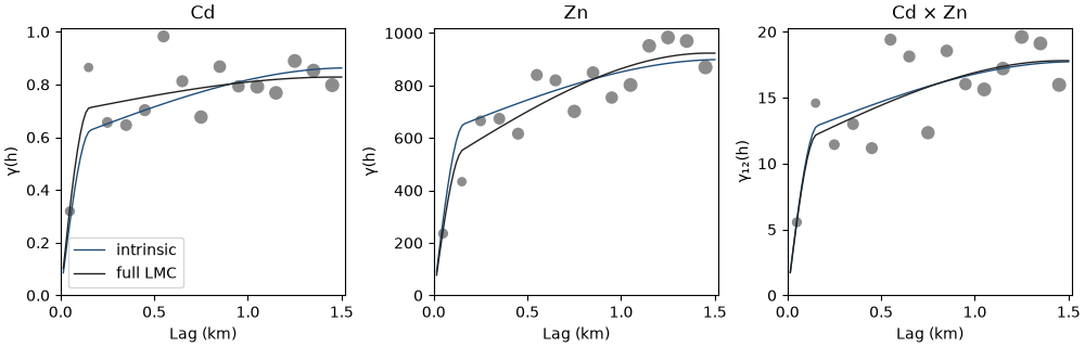
the full linear model of coregionalization of coregionalization gives each variable its own mix of the shared structures: Cd puts 83 % of its sill in the short structure, Zn 53 %. the intrinsic model gives both the same 68 %, a compromise, and one correlation, 0.64, at every lag. the total sills and the correlation differ little between the two models, so the curves meet at large lags. at short lags the intrinsic model is too smooth for Cd and too rough for Zn:
h = np.linspace(0, max_lag, 101)[1:]
origin = np.zeros((h.size, 3))
away = np.c_[h, np.zeros((h.size, 2))]
panels = ((0, 0, "Cd"), (1, 1, "Zn"), (0, 1, "Cd × Zn"))
fig, axes = plt.subplots(1, 3, figsize=(10, 3.2), layout="constrained")
for ax, (i, j, name) in zip(axes, panels):
    bt.plot.variogram(experimentals[i, j], ax=ax, color=GRAY)
    for model, color, label in [(icm, ACCENT, "intrinsic"), (lmc, INK, "full LMC")]:
        gamma = model.cross_covariance(i, j, origin, origin) - model.cross_covariance(i, j, origin, away)
        ax.plot(h, gamma, color=color, lw=1, label=label)
    ax.set(title=name, xlabel="Lag (km)", ylabel="γ(h)" if i == j else "γ₁₂(h)")
axes[0].legend()
save(fig, "variograms")
cokriging with either model
both models go to Cokriging the same way. the test kriges Cd at the 100 validation samples by collocated cokriging,
with Zn known there, as in cokriging. with correlations this close, the
simpler model predicts as well:
search = bt.Search(radius=1.5, max_samples=24, min_samples=4)
truth = test["Cd"]
for name, model in [("intrinsic", icm), ("full LMC", lmc)]:
    ck = bt.Cokriging(model, search, means=[cd.mean(), zn.mean()])
    ck.fit(np.vstack([xy, xy]), np.r_[cd, zn], [0] * len(cd) + [1] * len(zn))
    estimate = ck.predict(test, collocated={1: test["Zn"]})
    print(f"{name:>10}: validation RMSE {bt.compare(estimate, truth)['rmse']:.3f} mg/kg")
Out:
 intrinsic: validation RMSE 0.681 mg/kg
  full LMC: validation RMSE 0.689 mg/kg
seven metals
the intrinsic model grows with the number of variables only through its covariance matrix: seven metals need one shape and 28 matrix entries, fitted in one pass. its correlations hold at every lag:
metals = ["Cd", "Co", "Cr", "Cu", "Ni", "Pb", "Zn"]
seven = bt.Coregionalization.fit(
    bt.experimental_variograms(train, metals, lag, max_lag), ["spherical", "spherical"], intrinsic=True
)
c = sill(seven)
corr = c / np.sqrt(np.outer(np.diag(c), np.diag(c)))
print(f"smallest eigenvalue of the sill matrix {np.linalg.eigvalsh(c)[0]:.3g}")
print("      " + "".join(f"{m:>6}" for m in metals))
for m, row in zip(metals, corr):
    print(f"{m:<6}" + "".join(f"{r:6.2f}" for r in row))
Out:
smallest eigenvalue of the sill matrix 0.375
          Cd    Co    Cr    Cu    Ni    Pb    Zn
Cd      1.00  0.26  0.62  0.11  0.50  0.25  0.64
Co      0.26  1.00  0.52  0.30  0.74  0.24  0.53
Cr      0.62  0.52  1.00  0.23  0.73  0.31  0.69
Cu      0.11  0.30  0.23  1.00  0.28  0.79  0.60
Ni      0.50  0.74  0.73  0.28  1.00  0.36  0.67
Pb      0.25  0.24  0.31  0.79  0.36  1.00  0.63
Zn      0.64  0.53  0.69  0.60  0.67  0.63  1.00
Total running time of the script: ( 0 minutes 0.282 seconds)
Download Python source code: example_05_08.py