Note
Click here to download the full example code
cokriging
jura: 259 soil samples of heavy metals (mg/kg, coordinates in km) and 100 validation samples withheld from estimation. Cd correlates with Zn, and Zn is also known at the validation points, which suits collocated cokriging.
import sys
from pathlib import Path

HERE = Path(__file__).parent if "__file__" in globals() else Path.cwd()
sys.path.insert(0, str(HERE.parents[1]))
import boitata as bt
import matplotlib.pyplot as plt
import numpy as np
from common import ACCENT, GRAY, INK, save

train = bt.datasets.jura()["prediction"]
test = bt.datasets.jura()["validation"]
xy = train.coords
cd, zn = train["Cd"], train["Zn"]
lag, max_lag = 0.1, 1.5
a linear model of coregionalization with two spherical structures, fitted to the Cd and Zn variograms and their cross-variogram (coregionalization shows the fit), and an ordinary kriging of Cd alone for comparison:
experimentals = [
    [
        bt.experimental_variogram(xy, cd, lag, max_lag),
        bt.experimental_variogram(xy, cd, lag, max_lag, other=zn),
    ],
    [None, bt.experimental_variogram(xy, zn, lag, max_lag)],
]
lmc = bt.Coregionalization.fit(experimentals, ["spherical", "spherical"])
search = bt.Search(radius=1.5, max_samples=24, min_samples=4)
ok = bt.OrdinaryKriging(experimentals[0][0].fit("spherical"), search).fit(train, "Cd")
cokriging takes the samples of both variables with a variable index each. collocated cokriging also uses the secondary value at the target itself, here Zn at each validation point:
ck = bt.Cokriging(lmc, search, means=[cd.mean(), zn.mean()])
ck.fit(np.vstack([xy, xy]), np.r_[cd, zn], [0] * len(cd) + [1] * len(zn))
truth = test["Cd"]
by_ok = ok.predict(test)
by_ck = ck.predict(test, collocated={1: test["Zn"]})


def rmse(e):
    return bt.compare(e, truth)["rmse"]


print(f"validation RMSE: ordinary kriging {rmse(by_ok):.3f}, collocated cokriging {rmse(by_ck):.3f} mg/kg")
print(
    f"variance of estimates: ordinary kriging {by_ok.var():.3f}, cokriging {by_ck.var():.3f}, true {truth.var():.3f}"
)
Out:
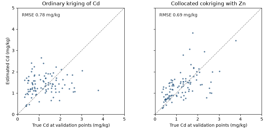
validation RMSE: ordinary kriging 0.777, collocated cokriging 0.689 mg/kg
variance of estimates: ordinary kriging 0.211, cokriging 0.531, true 0.477
using Zn at the target lowers the error and removes the smoothing that flattens ordinary kriging:
fig, axes = plt.subplots(1, 2, figsize=(9, 4.2), layout="constrained", sharey=True)
for ax, estimate, title in (
    (axes[0], by_ok, "Ordinary kriging of Cd"),
    (axes[1], by_ck, "Collocated cokriging with Zn"),
):
    ax.scatter(truth, estimate, s=12, color=ACCENT, alpha=0.7, linewidths=0)
    ax.plot([0, 5], [0, 5], color=GRAY, ls="--", lw=1)
    ax.set(xlim=(0, 5), ylim=(0, 5), xlabel="True Cd at validation points (mg/kg)", title=title)
    ax.set_aspect("equal")
    ax.text(0.2, 4.6, f"RMSE {rmse(estimate):.2f} mg/kg", color=INK)
axes[0].set_ylabel("Estimated Cd (mg/kg)")
save(fig, "validation")
locally varying anisotropy
anisotropy= takes a LocalAnisotropy as ordinary kriging does: each
target searches its own ellipse, shared by Cd and Zn, and every structure and cross term of the model turns with it.
here the directions follow the gradient of the ordinary kriging map of Cd, with semi-major ranges half the major.
collocated also takes a column of the targets by name:
grid = bt.BlockModel(origin=(0.3, 0.4), size=(0.1, 0.1), count=(47, 54))
guide = grid.with_column("Cd", ok.predict(grid))
lva = bt.LocalAnisotropy.from_grid(guide, "Cd", window=3, ratios=(0.5, 1.0)).smooth(0.5)
by_lva = ck.predict(test, anisotropy=lva, collocated={1: "Zn"})
print(
    f"validation RMSE: collocated cokriging {rmse(by_ck):.3f}, with local anisotropy {rmse(by_lva):.3f} mg/kg"
)
Out:
validation RMSE: collocated cokriging 0.689, with local anisotropy 0.671 mg/kg
Total running time of the script: ( 0 minutes 0.209 seconds)
Download Python source code: example_06_09.py