Note
Click here to download the full example code
From drill holes to a classified model
A resource estimate of three stacked sulphide lenses, end to end: drill-hole tables to composites inside each lens wireframe, declustered statistics and a capping check, the Zn variogram, a sub-blocked model built from the wireframes, Zn and density kriged in search passes, block-support simulation for risk, validation, classification, and tonnes and metal per lens saved to Parquet.
import sys
from pathlib import Path

HERE = Path(__file__).parent if "__file__" in globals() else Path.cwd()
sys.path.insert(0, str(HERE.parents[1]))
import tempfile

import boitata as bt
import matplotlib.pyplot as plt
import numpy as np
from common import ACCENT, GRAY, HIGHLIGHT, LIGHT, save
Drill holes
Collars, surveys and assays become desurveyed drill holes; each assay sits at the midpoint of its interval.
data = bt.datasets.stacked_sulphide_lenses()
drillholes = bt.Drillholes.from_tables(data)
samples = drillholes.samples()
print(f"{len(drillholes)} holes, {len(samples)} assays")
Out:
289 holes, 16995 assays
Samples inside each lens
Each lens wireframe is a closed mesh, so it has an inside. Each assay takes the name of the lens around its midpoint, and 2 m composites never cross from one lens to another or into the host rock.
lenses = {name: data[name] for name in ("lens_1", "lens_2", "lens_3")}
for name, mesh in lenses.items():
    print(f"{name}: closed {mesh.is_closed}, {mesh.volume / 1e6:.2f} Mm3")

lens = np.full(len(samples), "host", dtype=object)
for name, mesh in lenses.items():
    lens[mesh.contains(samples.coords)] = name
intervals = samples.with_columns({"LENS": list(lens)}).attributes
drillholes = bt.Drillholes(data["collars"], data["surveys"], intervals)
composites = drillholes.composite(2.0, ["ZN_PCT", "DENSITY"], domain="LENS", residual="merge")
composites = composites.filter(composites["LENS"] != "host")
names = composites["LENS"]
for name in lenses:
    inside = names == name
    measured = np.isfinite(composites["DENSITY"][inside]).sum()
    holes = len(set(composites["HOLE_ID"][inside]))
    print(f"{name}: {inside.sum()} composites from {holes} holes, {measured} with a density")
Out:
lens_1: closed True, 2.79 Mm3
lens_2: closed True, 1.90 Mm3
lens_3: closed True, 1.65 Mm3
lens_1: 609 composites from 78 holes, 408 with a density
lens_2: 279 composites from 53 holes, 234 with a density
lens_3: 263 composites from 49 holes, 200 with a density
Declustering and capping
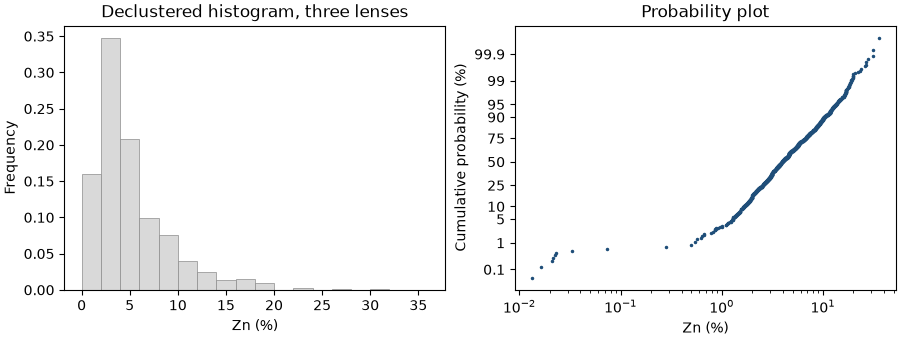
Holes cluster where a lens is rich, so each lens is cell-declustered on its own. The capping table then shows how much metal the top composites carry.
weights = np.zeros(len(composites))
for name in lenses:
    inside = names == name
    zn = composites["ZN_PCT"][inside]
    declustering = bt.cell_declustering(composites.coords[inside], zn, sizes=np.arange(10, 105, 5))
    weights[inside] = declustering.weights / declustering.weights.mean()
    print(
        f"{name}: mean {zn.mean():.2f} % Zn, declustered {declustering.mean:.2f} % ({declustering.cell_size:.0f} m cells)"
    )
composites = composites.with_column("weight", weights)

caps = bt.capping("ZN_PCT", weights="weight", data=composites)
for cap, fraction, removed in zip(caps["cap"], caps["fraction"], caps["metal_removed"], strict=True):
    print(f"cap {cap:5.1f} % Zn: {fraction:5.1%} of composites cut, {removed:5.1%} of the metal removed")

fig, (a, b) = plt.subplots(1, 2, figsize=(9, 3.4), layout="constrained")
bt.plot.histogram(
    "ZN_PCT", weights="weight", data=composites, bins=np.arange(0, 38, 2), ax=a, color=LIGHT, edgecolor=GRAY
)
a.set(xlabel="Zn (%)", title="Declustered histogram, three lenses")
bt.plot.probability("ZN_PCT", weights="weight", data=composites, log=True, ax=b, color=ACCENT, ms=3)
b.set(xlabel="Zn (%)", title="Probability plot")
save(fig, "statistics")
Out:
lens_1: mean 6.26 % Zn, declustered 5.22 % (90 m cells)
lens_2: mean 6.17 % Zn, declustered 5.24 % (40 m cells)
lens_3: mean 5.99 % Zn, declustered 5.17 % (80 m cells)
cap  10.3 % Zn: 10.0% of composites cut,  8.2% of the metal removed
cap  13.4 % Zn:  5.0% of composites cut,  3.8% of the metal removed
cap  16.6 % Zn:  2.5% of composites cut,  1.6% of the metal removed
cap  18.9 % Zn:  1.0% of composites cut,  0.9% of the metal removed
cap  21.8 % Zn:  0.5% of composites cut,  0.5% of the metal removed
cap  31.3 % Zn:  0.1% of composites cut,  0.0% of the metal removed
Declustering lowers every lens mean, most in lens 1. The top 1 % of composites, above 18.9 % Zn, holds 0.9 % of the metal, and the probability plot shows no break in the upper tail: leave the grades uncapped.
Zn variogram of lens 1
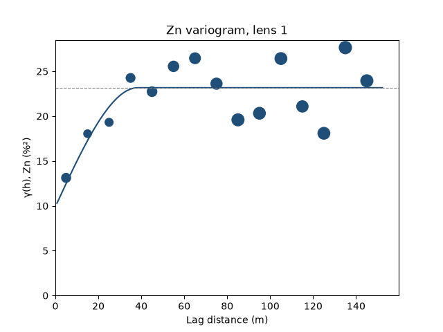
Lens 1 has the most composites. A thin lens leaves few pairs across it, so the variogram is omnidirectional; kriging uses the variogram of the grades, simulation that of the declustered normal scores, rescaled to a unit sill.
one = composites.filter(names == "lens_1")
grades = bt.experimental_variogram(one, "ZN_PCT", 10.0, 150.0)
variogram = grades.fit("spherical")
scores = bt.NormalScore().fit(one["ZN_PCT"], weights=one["weight"])
fitted = bt.experimental_variogram(one.coords, scores.transform(one["ZN_PCT"]), 10.0, 150.0).fit("spherical")
gaussian = fitted.standardized()
for label, model in (("Zn", variogram), ("normal scores", gaussian)):
    s = model.structures[0]
    print(f"{label}: nugget {model.nugget:.2f}, spherical sill {s.sill:.2f}, range {s.range:.0f} m")

fig, ax = bt.plot.variogram(grades, variogram=variogram, color=ACCENT)
ax.set(xlabel="Lag distance (m)", ylabel="γ(h), Zn (%²)", title="Zn variogram, lens 1")
save(fig, "variogram")
Out:
Zn: nugget 9.90, spherical sill 13.27, range 38 m
normal scores: nugget 0.49, spherical sill 0.51, range 43 m
A sub-blocked model
Parent blocks of 10 m are split into 5 m sub-blocks wherever a wireframe cuts them, so the model keeps each lens's volume; blocks outside every lens are dropped.
low = np.min([m.bounds[0] for m in lenses.values()], axis=0)
high = np.max([m.bounds[1] for m in lenses.values()], axis=0)
origin = np.floor(low / 10) * 10
count = [int(c) for c in np.ceil((high - origin) / 10)]
blocks = bt.BlockModel.from_meshes(
    origin, (10, 10, 10), count, [(mesh, "inside", name) for name, mesh in lenses.items()], 2, column="LENS"
)
block_lens = blocks["LENS"]
for name, mesh in lenses.items():
    volume = blocks.volumes[block_lens == name].sum()
    print(
        f"{name}: {np.sum(block_lens == name)} blocks, {volume / 1e6:.3f} Mm3 against {mesh.volume / 1e6:.3f} Mm3"
    )
Out:
lens_1: 7511 blocks, 2.789 Mm3 against 2.788 Mm3
lens_2: 6575 blocks, 1.900 Mm3 against 1.901 Mm3
lens_3: 5895 blocks, 1.651 Mm3 against 1.653 Mm3
Kriging in passes
Each lens is kriged from its own composites (domain_column). The first pass wants six composites within the
variogram range, at most two per hole, so at least three holes; blocks it leaves go to a pass at twice the range,
and a last one reaches every block. Two per hole matters here: holes with long intercepts tend to be the richer
ones, and would otherwise fill the search with their own composites. Density, measured on fewer samples, is
kriged the same way with the shape of the Zn variogram: kriging weights do not depend on the sill.
reach = variogram.structures[0].range
passes = [
    bt.Search(reach, max_samples=12, min_samples=6, max_per_hole=2),
    bt.Search(2 * reach, max_samples=12, min_samples=4, max_per_hole=2),
    bt.Search(250, max_samples=12, max_per_hole=2),
]
zn = bt.OrdinaryKriging(variogram, passes).fit(composites, "ZN_PCT", holes="HOLE_ID", domain_column="LENS")
kriged = zn.predict(blocks, diagnostics=True, domain_column="LENS")
measured = composites.drop_null("DENSITY")
density = bt.OrdinaryKriging(variogram, passes).fit(
    measured, "DENSITY", holes="HOLE_ID", domain_column="LENS"
)
blocks = blocks.with_columns(
    {
        "zn": kriged["value"],
        "density": density.predict(blocks, domain_column="LENS"),
        "pass": kriged["pass"],
        "slope": kriged["slope"],
    }
)
for p in (1, 2, 3):
    print(f"pass {p}: {np.mean(kriged['pass'] == p):.0%} of blocks")
print(f"density {np.nanmin(blocks['density']):.2f}-{np.nanmax(blocks['density']):.2f} t/m3")
Out:
pass 1: 8% of blocks
pass 2: 91% of blocks
pass 3: 1% of blocks
density 3.00-4.22 t/m3
Simulation at block support
Kriging smooths; the risk in a stope comes from simulation. Thirty sequential Gaussian simulations of lens 1
run on 5 m nodes, eight to each 10 m parent block the lens touches, and blocks= averages each realization
over those blocks, so the probability above 5 % Zn is that of a 10 m block. The first two kriging passes serve as
the simulation's search.
grid = bt.BlockModel(origin, (10, 10, 10), count)
parents = grid.filter(np.isin(np.arange(len(grid)), blocks.index[block_lens == "lens_1"]))
nodes = parents.discretize(2)
sgs = bt.SGS(gaussian, passes[:2]).fit(one, "ZN_PCT", weights="weight", holes="HOLE_ID")
summary = sgs.simulate(nodes, n=30, seed=1, cutoffs=[5.0], blocks=parents)
low, high = np.quantile(summary.realization_above[:, 0], [0.1, 0.9])
print(f"{len(parents)} parent blocks: P10 {low:.0%}, P90 {high:.0%} of them above 5 % Zn")
sure = np.mean(summary.probability_above[:, 0] > 0.9)
print(f"mean {summary.mean.mean():.2f} % Zn; blocks above 5 % in more than 90 % of realizations: {sure:.0%}")
Out:
4417 parent blocks: P10 43%, P90 50% of them above 5 % Zn
mean 5.30 % Zn; blocks above 5 % in more than 90 % of realizations: 1%
In eight realizations out of ten, between 42 and 51 % of the parent blocks exceed 5 % Zn, yet only 1 % of them do so in more than 90 % of the realizations: at this drill spacing few single blocks are certain ore, although the share of ore across the lens is well known.
Validation
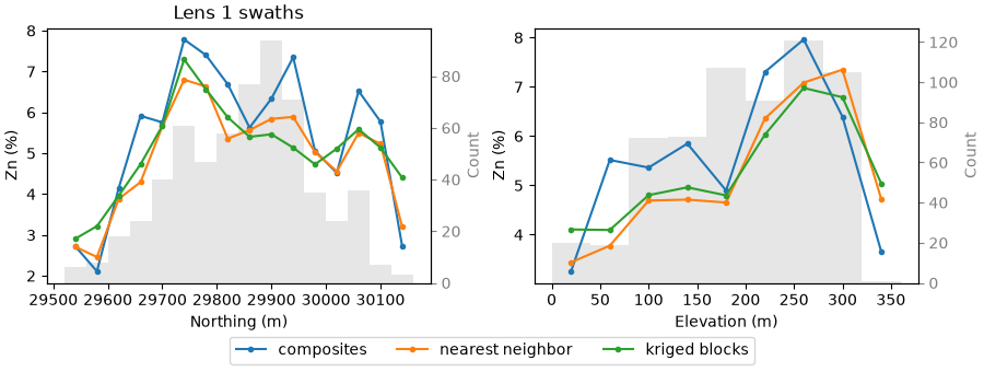
The kriged blocks, weighted by volume, should match the declustered composites of each lens, and a nearest-neighbor model, the other unbiased reference, and follow them along strike and down the lens.
nearest = bt.NearestNeighbor(bt.Search(250, max_samples=1)).fit(composites, "ZN_PCT", domain_column="LENS")
blocks = blocks.with_column("nn", nearest.predict(blocks, domain_column="LENS"))
for name in lenses:
    inside = block_lens == name
    bias = bt.global_bias(
        blocks["zn"][inside],
        composites["ZN_PCT"][names == name],
        weights=blocks.volumes[inside],
        data_weights=weights[names == name],
    )
    nn = np.average(blocks["nn"][inside], weights=blocks.volumes[inside])
    print(
        f"{name}: kriged {bias['estimate_mean']:.2f} % Zn, declustered composites {bias['data_mean']:.2f} % "
        f"({bias['relative']:+.1%}), nearest neighbor {nn:.2f} % ({bias['estimate_mean'] / nn - 1:+.1%})"
    )

in_one = blocks.filter(block_lens == "lens_1")
fig, axes = plt.subplots(1, 2, figsize=(9, 3.4), layout="constrained")
for ax, (axis, label) in zip(axes, (("y", "Northing (m)"), ("z", "Elevation (m)")), strict=True):
    bt.plot.swath(
        [
            bt.swath(one, "ZN_PCT", 40.0, axis=axis),
            bt.swath(in_one, "nn", 40.0, axis=axis, weights=in_one.volumes),
            bt.swath(in_one, "zn", 40.0, axis=axis, weights=in_one.volumes),
        ],
        labels=["composites", "nearest neighbor", "kriged blocks"],
        ax=ax,
    )
    ax.set(xlabel=label, ylabel="Zn (%)")
    ax.get_legend().remove()
axes[0].set_title("Lens 1 swaths")
fig.legend(*axes[0].get_legend_handles_labels(), loc="outside lower center", ncol=3)
save(fig, "swath")
Out:
lens_1: kriged 5.49 % Zn, declustered composites 5.22 % (+5.3%), nearest neighbor 5.50 % (-0.1%)
lens_2: kriged 5.46 % Zn, declustered composites 5.24 % (+4.2%), nearest neighbor 4.88 % (+11.8%)
lens_3: kriged 5.30 % Zn, declustered composites 5.17 % (+2.5%), nearest neighbor 4.48 % (+18.3%)
In lens 1 the kriged mean equals that of the nearest-neighbor model and lies 5.3 % above the declustered composites; in lenses 2 and 3 it is 4 and 3 % above the declustered composites but 12 and 18 % above nearest neighbor. The two references disagree with each other as much as with the model: nearest neighbor spreads each edge composite over the blocks around it, and cell declustering depends on the cell size it settles on. Along northing and elevation, kriged blocks and nearest neighbor follow the same course, and the composites swing around both, as raw data do.
Classification
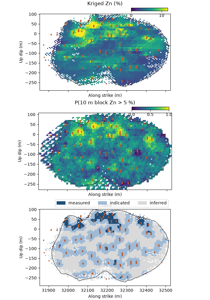
Measured blocks come from the first pass with a slope of regression of at least 0.6; indicated, from the first two passes with a slope of 0.3; the rest is inferred. With a nugget of 43 % of the sill and a 38 m range, only blocks close to several holes qualify as measured.
rules = [
    ("measured", {"pass": ("<=", 1), "slope": (">=", 0.6)}),
    ("indicated", {"pass": ("<=", 2), "slope": (">=", 0.3)}),
]
classes = bt.classify(kriged, rules, default="inferred")
categories = bt.Categories(["measured", "indicated", "inferred"], colors=[ACCENT, "#9ebad6", LIGHT])
blocks = blocks.with_column("class", categories.encode(classes))
for name in categories.names:
    print(f"{name:>9}: {np.mean(classes == name):.0%} of blocks")
Out:
 measured: 2% of blocks
indicated: 39% of blocks
 inferred: 59% of blocks
Lens 1 is seen face on, on the plane through its middle, with its outline on that plane and its composites as dots. The plane's pole is the least spread direction of the wireframe's vertices.
parents = parents.with_column("p_above_5", summary.probability_above[:, 0])
vertices = lenses["lens_1"].coords
pole = np.linalg.eigh(np.cov(vertices.T))[1][:, 0]
pole *= np.sign(pole[2])
strike = (np.degrees(np.arctan2(pole[0], pole[1])) - 90) % 360
dip = np.degrees(np.arccos(pole[2]))
print(f"lens 1 strikes {strike:03.0f}°, dips {dip:.0f}°")
plane = (tuple(vertices.mean(axis=0)), strike, dip)
fig, axes = plt.subplots(3, 1, figsize=(7, 10), layout="constrained", sharex=True)
bt.plot.section(blocks, "zn", plane=plane, ax=axes[0], colorbar=False, vmin=0, vmax=12)
bt.plot.section(parents, "p_above_5", plane=plane, ax=axes[1], colorbar=False, vmin=0, vmax=1)
bt.plot.section(blocks, "class", plane=plane, ax=axes[2], colorbar=False, scheme=categories)
for ax in axes[:2]:
    fig.colorbar(ax.images[0], cax=ax.inset_axes([0.7, 1.04, 0.28, 0.04]), orientation="horizontal")
bt.plot.category_legend(categories, axes[2], loc="lower right", bbox_to_anchor=(1, 1), ncol=3)
titles = ("Kriged Zn (%)", "P(10 m block Zn > 5 %)", "Class")
for ax, title in zip(axes, titles, strict=True):
    bt.plot.slab(one, plane=plane, thickness=60, meshes=[lenses["lens_1"]], s=3, color=HIGHLIGHT, ax=ax)
    ax.set(title=title, aspect="equal")
save(fig, "section")
Out:
lens 1 strikes 021°, dips 59°
Tonnes and metal
Tonnes are block volume × kriged density and metal is tonnes × Zn, per lens and class, in all of each lens and above a 5 % Zn cutoff.
print(f"{'':20}{'kt':>8}{'Zn %':>7}{'kt Zn':>8}")
for groups in (block_lens, classes):
    table = bt.grade_tonnage(
        "zn", [0.0, 5.0], weights=blocks.volumes, density="density", categories=groups, data=blocks
    )
    for category, cutoff, tonnes, grade, metal in zip(
        *(table[c] for c in ("category", "cutoff", "tonnage", "mean_grade", "metal")), strict=True
    ):
        print(f"{category:10} ≥ {cutoff:1.0f} % Zn{tonnes / 1e3:8.0f}{grade:7.2f}{metal / 1e5:8.1f}")
Out:
                          kt   Zn %   kt Zn
lens_1     ≥ 0 % Zn    9564   5.55   530.4
lens_1     ≥ 5 % Zn    4700   7.31   343.4
lens_2     ≥ 0 % Zn    6412   5.51   353.4
lens_2     ≥ 5 % Zn    3566   7.01   249.9
lens_3     ≥ 0 % Zn    5531   5.33   294.9
lens_3     ≥ 5 % Zn    2974   6.38   189.7
all        ≥ 0 % Zn   21507   5.48  1178.7
all        ≥ 5 % Zn   11241   6.97   783.0
indicated  ≥ 0 % Zn    8681   5.73   497.1
indicated  ≥ 5 % Zn    4803   7.26   348.8
inferred   ≥ 0 % Zn   12198   5.21   635.3
inferred   ≥ 5 % Zn    6021   6.58   396.0
measured   ≥ 0 % Zn     628   7.38    46.4
measured   ≥ 5 % Zn     417   9.15    38.2
all        ≥ 0 % Zn   21507   5.48  1178.7
all        ≥ 5 % Zn   11241   6.97   783.0
The three lenses hold 21.5 Mt at 5.48 % Zn, 1.18 Mt of zinc, of which 11.2 Mt at 6.97 % lie above 5 % Zn. Lens 1 carries 45 % of the metal; measured blocks, only 628 kt, are its rich core near the top.
The model, sub-blocks, lens names, grades, classes and all, goes to Parquet and back unchanged.
with tempfile.TemporaryDirectory() as folder:
    path = Path(folder) / "lenses.parquet"
    bt.write_parquet(path, blocks)
    stored = bt.read_parquet(path)
print(f"{len(stored)} blocks, columns {stored.column_names}")
same = np.array_equal(stored.extents, blocks.extents) and np.array_equal(stored["zn"], blocks["zn"])
print(f"same sub-blocks and Zn: {same}")
Out:
19981 blocks, columns ['LENS', 'zn', 'density', 'pass', 'slope', 'nn', 'class']
same sub-blocks and Zn: True
Total running time of the script: ( 0 minutes 1.367 seconds)
Download Python source code: example_12_02.py