turning bands¶

turning bands sums many one-dimensional processes along random lines into an unconditional gaussian field, then conditions it to the data by kriging the residuals. it draws the same kind of realizations as SGS (sequential gaussian simulation) without a random path.

import sys
import time
from pathlib import Path

HERE = Path(__file__).parent if "__file__" in globals() else Path.cwd()
sys.path.insert(0, str(HERE.parents[1]))

import boitata as bt
import matplotlib.pyplot as plt
import numpy as np
from common import GRAY, HIGHLIGHT, LIGHT, map_axes, save
from matplotlib.colors import PowerNorm

samples = bt.datasets.walker_lake()
xy, v = samples.coords, samples["V"]
grid = bt.BlockModel(origin=(0.5, 0.5), size=(5, 5), count=(52, 60))

declustered normal scores and their variogram along N170°, the direction of greatest continuity (variogram fitting), and across it, scaled to a unit sill:

weights = bt.cell_declustering(xy, v, sizes=np.arange(2.5, 102.5, 2.5)).weights
y = bt.NormalScore(tails=(0.0, v.max())).fit_transform(v, weights=weights)
major = bt.experimental_variogram(xy, y, 10.0, 120.0, azimuth=170).fit("spherical")
minor = bt.experimental_variogram(xy, y, 10.0, 120.0, azimuth=260).fit("spherical")
ratio = min(minor.structures[0].range / major.structures[0].range, 1.0)
gaussian = major.standardized().with_anisotropy((170, 0, 0), (ratio, 1.0))
print(gaussian)

Out:

Variogram(nugget=0.3315861183518779, structures=[Structure("spherical", sill=0.6684138816481222, range=82.43111673409601)], rotation=(170.0, 0.0, 0.0), ratios=(0.42564072265384956, 1.0))

both methods normal-score the data, simulate and back-transform; bands sets how many lines turning bands sums.

sgs = bt.SGS(gaussian, bt.Search(radius=100, max_samples=24)).fit(samples, "V", weights=weights)
tb = bt.TurningBands(gaussian, bands=500).fit(samples, "V", weights=weights)
start = time.perf_counter()
by_sgs = sgs.simulate(grid, n=20, seed=5, keep=True).realizations
sgs_seconds = time.perf_counter() - start
start = time.perf_counter()
by_tb = tb.simulate(grid, n=20, seed=5, keep=True).realizations
tb_seconds = time.perf_counter() - start
for name, reals, seconds in (("SGS", by_sgs, sgs_seconds), ("turning bands", by_tb, tb_seconds)):
    print(
        f"{name:>13}: 20 realizations in {seconds:.2f} s, mean {reals.mean():.0f} ppm, variance {reals.var():.0f} ppm²"
    )

Out:

          SGS: 20 realizations in 0.02 s, mean 300 ppm, variance 71089 ppm²
turning bands: 20 realizations in 0.09 s, mean 295 ppm, variance 69672 ppm²

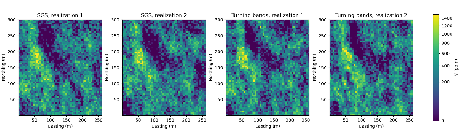
both follow the same high-grade trends, with the same short-scale scatter:

extent = (0.5, 260.5, 0.5, 300.5)
norm = PowerNorm(0.5, vmin=0, vmax=1500)
fig, axes = plt.subplots(1, 4, figsize=(15, 4.4), layout="constrained")
panels = [
    (by_sgs[0], "SGS, realization 1"),
    (by_sgs[1], "SGS, realization 2"),
    (by_tb[0], "Turning bands, realization 1"),
    (by_tb[1], "Turning bands, realization 2"),
]
for ax, (image, title) in zip(axes, panels):
    im = ax.imshow(grid.grid(image)[0], origin="lower", extent=extent, norm=norm)
    map_axes(ax, title)
fig.colorbar(im, ax=axes, shrink=0.8, label="V (ppm)")
save(fig, "realizations")

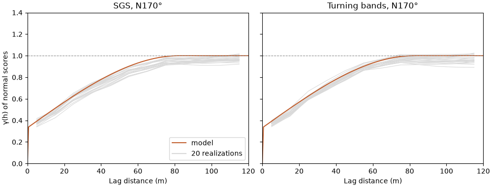
SGS, realization 1, SGS, realization 2, Turning bands, realization 1, Turning bands, realization 2

along the major axis both follow the model, from its nugget at the first lags to the sill at its range. turning bands simulates the nugget as independent noise at each node, since the bands carry only the structures:

h = np.linspace(0, 120, 200)
fig, axes = plt.subplots(1, 2, figsize=(10, 3.8), layout="constrained", sharey=True)
for ax, (name, reals) in zip(axes, (("SGS", by_sgs), ("Turning bands", by_tb))):
    for r in reals:
        scores = bt.NormalScore().fit_transform(r)
        exp = bt.experimental_variogram(grid.coords, scores, 10.0, 120.0, azimuth=170)
        ax.plot(exp.lags, exp.gammas, color=LIGHT, lw=0.8)
    ax.plot(h, gaussian.gamma(h), color=HIGHLIGHT, lw=1.4, label="model")
    ax.plot([], [], color=LIGHT, label="20 realizations")
    ax.axhline(1.0, color=GRAY, lw=0.8, ls="--")
    ax.set(xlim=(0, 120), ylim=(0, 1.4), xlabel="Lag distance (m)", title=f"{name}, N170°")
axes[0].set_ylabel("γ(h) of normal scores")
axes[0].legend(loc="lower right")
save(fig, "variograms")