soft boundaries¶

a laterite grades from limonite (LIM) down into saprolite (SAP), and nickel shows no sharp step at the logged contact. fitted with domains= or domain_column=, an estimator informs each target from samples of its own domain only: a hard boundary. Search(..., soft=...) opens it, so samples of another domain within the soft distance inform a target too, both ways or, with a dict, one way only. kriging and SGS take the same search.

import sys
from pathlib import Path

HERE = Path(__file__).parent if "__file__" in globals() else Path.cwd()
sys.path.insert(0, str(HERE.parents[1]))

import boitata as bt
import matplotlib.pyplot as plt
import numpy as np
from common import ACCENT, GRAY, HIGHLIGHT, INK, save

data = bt.datasets.nickel_laterite_profile()
intervals = bt.merge_intervals(data["assays"], data["horizons"])
samples = bt.Drillholes(data["collars"], data["surveys"], intervals).samples()
samples = samples.filter(np.isin(samples["HORIZON"], ["LIM", "SAP"]))
horizon = samples["HORIZON"]
for name in ("LIM", "SAP"):
    print(
        f"{name}: {np.sum(horizon == name)} samples of 1 m, mean {samples['NI_PCT'][horizon == name].mean():.2f} % Ni"
    )


def profile(points, values):
    return bt.contact(
        points,
        values,
        domain_column="HORIZON",
        holes="HOLE_ID",
        inside="SAP",
        outside="LIM",
        max_distance=7.0,
        bin=1,
    )

Out:

LIM: 3334 samples of 1 m, mean 1.08 % Ni
SAP: 4901 samples of 1 m, mean 1.81 % Ni

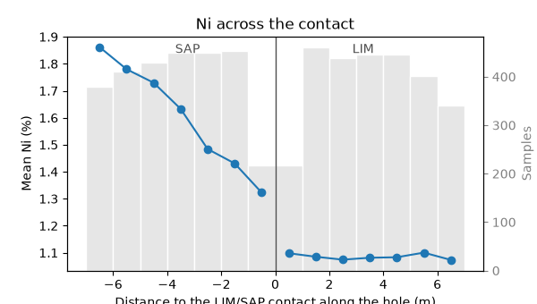
down each hole, the mean grade against the distance to the LIM/SAP contact:

observed = profile(samples, "NI_PCT")
print("distance:", observed["distance"])
print("mean Ni: ", observed["mean"].round(2))

fig, ax = bt.plot.contact(observed, labels=("SAP", "LIM"))
fig.set_size_inches(6, 3.4)
ax.set(
    xlabel="Distance to the LIM/SAP contact along the hole (m)",
    ylabel="Mean Ni (%)",
    title="Ni across the contact",
)
save(fig, "contact")

Ni across the contact

Out:

distance: [-6.5 -5.5 -4.5 -3.5 -2.5 -1.5 -0.5  0.5  1.5  2.5  3.5  4.5  5.5  6.5]
mean Ni:  [1.86 1.78 1.73 1.63 1.48 1.43 1.32 1.1  1.09 1.07 1.08 1.08 1.1  1.07]

LIM is flat up to the contact. SAP loses grade toward it, from 1.86 % Ni 6 to 7 m below to 1.32 % in the last meter, and the step at the contact itself is small: the boundary is gradational on the saprolite side.

one normal-score variogram serves both horizons: each is scored on its own, then the scores are pooled. the nugget and vertical range come from pairs down the holes, the horizontal range from pairs across them. kriging weights do not depend on the sill, so the same model serves kriging and SGS.

scores = np.empty(len(samples))
for name in ("LIM", "SAP"):
    scores[horizon == name] = bt.NormalScore().fit_transform(samples["NI_PCT"][horizon == name])
down = bt.experimental_variogram(samples, scores, 1, 12, holes="HOLE_ID").fit("spherical")
across = bt.experimental_variogram(samples, scores, 25, 250, azimuth=0, tolerance=22.5).fit(
    "spherical", nugget=down.nugget
)
model = across.with_anisotropy((0, 0, 0), (1.0, down.structures[0].range / across.structures[0].range))
print(model)

Out:

Variogram(nugget=0.32861112557336725, structures=[Structure("spherical", sill=0.6938819610021464, range=54.74522060744121)], rotation=(0.0, 0.0, 0.0), ratios=(1.0, 0.13561192309647335))

the holes on the 50 m mesh do the estimating; the 25 m infill holes are held out to check it. three rules share one search, flattened ten to one, near the seven to one of the variogram. the soft distance is measured in that ellipsoid, so 50 reaches 50 m across and 5 m up or down, most of the transition. the one-way rule lets SAP draw on LIM but not the other way round.

collars = data["collars"]
offset = [np.abs((collars[axis] + 25) % 50 - 25) for axis in ("X", "Y")]
infill = collars["HOLE_ID"][(offset[0] > 12) | (offset[1] > 12)]
held_out = np.isin(samples["HOLE_ID"], infill)
mesh, check = samples.filter(~held_out), samples.filter(held_out)
print(f"{len(collars) - len(infill)} mesh holes, {len(infill)} infill holes held out")

rules = {"hard": None, "soft both ways": 50.0, "soft, SAP from LIM": {("SAP", "LIM"): 50.0}}
searches = {
    name: bt.Search(200, max_samples=24, min_samples=4, max_per_hole=6, ratios=(1.0, 0.1), soft=soft)
    for name, soft in rules.items()
}
truth = check["NI_PCT"]
check_horizon = check["HORIZON"]
kriged = {}
for name, search in searches.items():
    ok = bt.OrdinaryKriging(model, search).fit(mesh, "NI_PCT", holes="HOLE_ID", domain_column="HORIZON")
    result = ok.predict(check, diagnostics=True, domain_column="HORIZON")
    kriged[name] = result["value"]
    error = result["value"] - truth
    rmse = {h: np.sqrt(np.mean(error[check_horizon == h] ** 2)) for h in ("LIM", "SAP")}
    other = {h: np.mean(result["n_other_domain"][check_horizon == h] > 0) for h in ("LIM", "SAP")}
    print(
        f"{name:>18}: RMSE LIM {rmse['LIM']:.3f}, SAP {rmse['SAP']:.3f}; "
        f"other horizon used by {other['LIM']:.0%} of LIM, {other['SAP']:.0%} of SAP targets"
    )

Out:

301 mesh holes, 147 infill holes held out
              hard: RMSE LIM 0.410, SAP 0.774; other horizon used by 0% of LIM, 0% of SAP targets
    soft both ways: RMSE LIM 0.424, SAP 0.770; other horizon used by 70% of LIM, 42% of SAP targets
soft, SAP from LIM: RMSE LIM 0.410, SAP 0.770; other horizon used by 0% of LIM, 42% of SAP targets

most targets lie far from the contact, so the errors change little. the mean estimate by distance to the contact shows where the rules differ:

def means(values):
    return profile(check, values)["mean"].round(2)


distance = profile(check, "NI_PCT")["distance"]
print(f"{'distance':>18}:", distance)
print(f"{'held out':>18}:", means("NI_PCT"))
for name, values in kriged.items():
    print(f"{name:>18}:", means(values))

Out:

          distance: [-6.5 -5.5 -4.5 -3.5 -2.5 -1.5 -0.5  0.5  1.5  2.5  3.5  4.5  5.5  6.5]
          held out: [1.84 1.77 1.68 1.57 1.44 1.36 1.28 1.06 1.05 1.06 1.05 1.05 1.   1.01]
              hard: [1.89 1.84 1.76 1.68 1.61 1.57 1.55 1.03 1.04 1.05 1.05 1.06 1.06 1.08]
    soft both ways: [1.88 1.81 1.71 1.59 1.48 1.39 1.34 1.21 1.18 1.13 1.1  1.09 1.08 1.09]
soft, SAP from LIM: [1.88 1.81 1.71 1.59 1.48 1.39 1.34 1.03 1.04 1.05 1.05 1.06 1.06 1.08]

SGS takes the same searches and the same domains. each horizon keeps its own normal-score table; a LIM sample informing a SAP node enters by its grade, scored through the SAP table. the mean of 20 realizations at the held-out samples:

simulated = {}
for name, search in searches.items():
    sgs = bt.SGS(model, search).fit(mesh, "NI_PCT", holes="HOLE_ID", domain_column="HORIZON")
    simulated[name] = sgs.simulate(check, n=20, seed=7, domain_column="HORIZON").mean
    print(f"{name:>18}:", means(simulated[name]))

Out:

              hard: [1.84 1.8  1.74 1.67 1.64 1.61 1.6  1.05 1.07 1.09 1.08 1.08 1.1  1.11]
    soft both ways: [1.8  1.74 1.64 1.53 1.44 1.35 1.31 1.25 1.23 1.2  1.16 1.13 1.13 1.13]
soft, SAP from LIM: [1.79 1.73 1.63 1.5  1.4  1.29 1.24 1.05 1.07 1.09 1.08 1.08 1.1  1.11]

styles = {"hard": (GRAY, "-"), "soft both ways": (HIGHLIGHT, "--"), "soft, SAP from LIM": (ACCENT, "-")}
fig, axes = plt.subplots(1, 2, figsize=(9.6, 3.6), sharey=True, layout="constrained")
for ax, estimates, title in ((axes[0], kriged, "Ordinary kriging"), (axes[1], simulated, "SGS, mean of 20")):
    for i, side in enumerate((distance < 0, distance > 0)):
        ax.plot(
            distance[side],
            means("NI_PCT")[side],
            "o",
            color=INK,
            ms=4,
            label=None if i else "held-out samples",
        )
        for name, values in estimates.items():
            color, style = styles[name]
            ax.plot(distance[side], means(values)[side], ls=style, color=color, label=None if i else name)
    ax.axvline(0, color=GRAY, lw=0.8)
    ax.set(title=title, xlabel="Distance to the contact (m), SAP < 0 < LIM")
axes[0].set_ylabel("Mean Ni (%)")
axes[1].legend(loc="upper right")
save(fig, "profiles")

Ordinary kriging, SGS, mean of 20

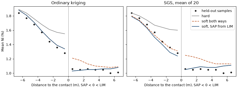
in the last meter of SAP the hard boundary kriges 1.55 % Ni against 1.28 % held out: it sees only saprolite, richer deeper down. letting SAP draw on LIM brings it to 1.34 % and follows the gradient. opened both ways, the boundary also lifts the first meter of LIM from 1.03 % to 1.21 %, where the held-out samples stay at 1.06 %. SGS agrees: 1.60 % hard and 1.24 % one way in the last meter of SAP, and 1.25 % in the first meter of LIM when soft both ways. the contact profile says which way to open a boundary; here only the saprolite side is gradational.

Total running time of the script: ( 0 minutes 0.686 seconds)

Download Python source code: example_06_13.py

Download Jupyter notebook: example_06_13.ipynb

Gallery generated by mkdocs-gallery