search calibration¶

calibrate_search scores candidate searches for block kriging of walker lake V on 10 × 10 m blocks, keeping the variogram and samples. it picks no winner, and the exhaustive grid checks every score.

import sys
from pathlib import Path

HERE = Path(__file__).parent if "__file__" in globals() else Path.cwd()
sys.path.insert(0, str(HERE.parents[1]))

import boitata as bt
import matplotlib.pyplot as plt
import numpy as np
from common import ACCENT, GRAY, save

samples = bt.datasets.walker_lake()
truth = bt.datasets.walker_lake_exhaustive()["V"].reshape(300, 260)
xy, v = samples.coords, samples["V"]
azimuths = np.arange(0, 180, 22.5)
directional = [bt.experimental_variogram(xy, v, 10.0, 120.0, azimuth=a) for a in azimuths]
model = bt.Variogram.fit_directional(
    directional, [(a, 0) for a in azimuths], ["spherical", "spherical"], weighting="count/gamma"
)
weights = bt.cell_declustering(xy, v, sizes=np.arange(2.5, 102.5, 2.5)).weights

blocks = bt.BlockModel(origin=(0.5, 0.5), size=(10, 10), count=(26, 30))
search = bt.Search(radius=80, max_samples=24, min_samples=4, rotation=model.rotation, ratios=(0.5, 1.0))
kriging = bt.BlockKriging(model, search, size=(10, 10), discretization=(5, 5, 1)).fit(xy, v)
true_blocks = truth.reshape(30, 10, 26, 10).mean(axis=(1, 3)).ravel()

each candidate re-estimates the blocks and gets scores for the variance of the estimates against the block variance (sill minus the mean variogram within a block, nugget excluded), slope and efficiency (mean and 10th percentile), negative weights, the share of blocks each pass fills, declustered cross-validation at the samples (cross-validation), and the global bias. with cutoffs and a hermite anamorphosis it adds tonnage and metal above each cutoff, against those of the discrete gaussian model's block distribution (discrete gaussian model). here the candidates differ only in max_samples.

counts = (4, 8, 12, 16, 24, 32, 48)
candidates = [
    bt.Search(radius=80, max_samples=n, min_samples=4, rotation=model.rotation, ratios=(0.5, 1.0))
    for n in counts
]
anamorphosis = bt.HermiteAnamorphosis().fit(v, weights=weights)
scores = bt.calibrate_search(
    kriging, candidates, blocks, weights=weights, cutoffs=[500], anamorphosis=anamorphosis
)
true_scores = {"slope": [], "variance": [], "tonnage": []}
for candidate in candidates:
    estimate = kriging.with_search(candidate).predict(blocks)
    true_scores["slope"].append(bt.compare(estimate, true_blocks)["slope"])
    true_scores["variance"].append(estimate.var() / true_blocks.var())
    true_scores["tonnage"].append(np.mean(estimate >= 500) / np.mean(true_blocks >= 500))
print(f"{'':7} {'slope of regression':^20} {'variance ratio':^13} {'tonnage >= 500':^13} {'negative':>8}")
print(
    f"{'samples':>7}"
    + "".join(f"{h:>7}" for h in ("mean", "CV", "true", "scores", "true", "scores", "true"))
    + "  weights"
)
for i, n in enumerate(counts):
    row = (scores["slope_mean"][i], scores["cv_slope"][i], true_scores["slope"][i])
    row += (scores["variance_ratio"][i], true_scores["variance"][i])
    row += (scores["tonnage_ratio_500"][i], true_scores["tonnage"][i])
    print(f"{n:7d}" + "".join(f"{x:7.2f}" for x in row) + f"{scores['negative_weight_sum'][i]:9.3f}")

Out:

        slope of regression  variance ratio tonnage >= 500 negative
samples   mean     CV   true scores   true scores   true  weights
      4   0.84   0.89   0.93   0.75   0.91   1.03   0.97    0.000
      8   0.92   0.97   0.99   0.67   0.81   0.94   0.88   -0.001
     12   0.94   0.99   1.01   0.64   0.77   0.91   0.85   -0.006
     16   0.95   1.00   1.02   0.62   0.76   0.88   0.83   -0.012
     24   0.96   1.01   1.02   0.62   0.75   0.85   0.79   -0.022
     32   0.96   1.01   1.02   0.62   0.76   0.85   0.79   -0.029
     48   0.97   1.01   1.02   0.62   0.75   0.85   0.79   -0.037

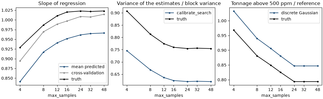
every score moves with the truth. more samples raise the slope, and the cross-validation slope follows the true one; the mean predicted slope sits lower. estimates grow smoother, so the variance ratio falls and fewer blocks clear 500 ppm. the true variance ratio sits higher because the blocks of this 260 × 300 m area vary less than the sill implies, and the discrete gaussian reference puts about 7 % fewer blocks above 500 ppm than the truth. past 16 to 24 samples the slope rises little while the negative weights keep growing; you settle that trade-off.

fig, axes = plt.subplots(1, 3, figsize=(11, 3.4), layout="constrained")
panels = (
    (
        "Slope of regression",
        [(scores["slope_mean"], "mean predicted"), (scores["cv_slope"], "cross-validation")],
        "slope",
    ),
    (
        "Variance of the estimates / block variance",
        [(scores["variance_ratio"], "calibrate_search")],
        "variance",
    ),
    ("Tonnage above 500 ppm / reference", [(scores["tonnage_ratio_500"], "discrete Gaussian")], "tonnage"),
)
for ax, (title, lines, key) in zip(axes, panels, strict=True):
    for (series, label), color in zip(lines, (ACCENT, GRAY), strict=False):
        ax.plot(counts, series, "o-", color=color, label=label, ms=3)
    ax.plot(counts, true_scores[key], "o-", color="black", label="truth", ms=3)
    ax.set(title=title, xlabel="max_samples", xscale="log", xticks=counts, xticklabels=counts)
    ax.minorticks_off()
    ax.legend()
save(fig, "calibration")

Slope of regression, Variance of the estimates / block variance, Tonnage above 500 ppm / reference

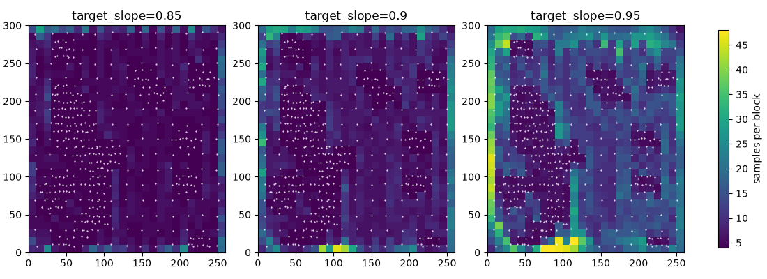
calibrate_search picks one search for every block. a search with target_slope (or target_efficiency) calibrates block by block instead: each block takes the fewest samples, from min_samples up, whose slope of regression reaches the target, and max_samples where none does. the diagnostics' target_met flags which. well-informed blocks keep few samples and stay sharp, and sparse ones gather more.

print(f"{'target':>7} {'samples':>8} {'met':>6} {'true slope':>11} {'variance ratio':>15}")
local = {}
for target in (0.85, 0.9, 0.95):
    calibrated = bt.Search(
        radius=80,
        max_samples=48,
        min_samples=4,
        rotation=model.rotation,
        ratios=(0.5, 1.0),
        target_slope=target,
    )
    d = kriging.with_search(calibrated).predict(blocks, diagnostics=True)
    local[target] = d["n_samples"]
    estimate = d["value"]
    print(
        f"{target:7.2f} {d['n_samples'].mean():8.1f} {np.mean(d['target_met'] == 1):6.0%}"
        f" {bt.compare(estimate, true_blocks)['slope']:11.2f} {estimate.var() / true_blocks.var():15.2f}"
    )

Out:

 target  samples    met  true slope  variance ratio
   0.85      5.7    98%        0.95            0.87
   0.90      8.4    92%        0.97            0.84
   0.95     14.4    82%        1.00            0.78

a higher target takes more samples, raises the true slope and smooths more, as a larger fixed search does. at about the same mean count as a fixed search, the calibrated one smooths a little less for a slightly lower slope. it sends the samples where the drilling is sparse: the dense clusters keep the minimum, the edges and gaps take the most, and a few edge blocks fall short even at max_samples.

fig, axes = plt.subplots(1, 3, figsize=(11, 4), layout="constrained")
for ax, (target, n) in zip(axes, local.items(), strict=True):
    image = ax.imshow(
        blocks.grid(n)[0], origin="lower", extent=(0, 260, 0, 300), vmin=4, vmax=48, cmap="viridis"
    )
    ax.plot(xy[:, 0], xy[:, 1], ".", color="white", ms=1)
    ax.set(title=f"target_slope={target}", aspect="equal")
fig.colorbar(image, ax=axes, shrink=0.8, label="samples per block")
save(fig, "local")