Note
Click here to download the full example code
soft-boundary statistics
contact() (contacts) showed nickel tapering into the LIM/SAP
contact without a step: a gradational, soft boundary. soft boundaries
opens the search of SAP to LIM samples within 50 m. soft_boundary() measures what that buffer draws in: SAP
statistics computed alone (hard) against statistics that also fold in LIM samples within the buffer of their nearest
SAP sample (soft).
import sys
from pathlib import Path

HERE = Path(__file__).parent if "__file__" in globals() else Path.cwd()
sys.path.insert(0, str(HERE.parents[1]))
import boitata as bt
import matplotlib.pyplot as plt
import numpy as np
from common import ACCENT, GRAY, save

data = bt.datasets.nickel_laterite_profile()
intervals = bt.merge_intervals(data["assays"], data["horizons"])
samples = bt.Drillholes(data["collars"], data["surveys"], intervals).samples()
samples = samples.filter(np.isin(samples["HORIZON"], ["LIM", "SAP"]))
contact put Ni at 1.10 % just outside the LIM/SAP contact and 1.32 % just inside, still climbing several meters into
the saprolite. that gradation is why soft boundaries opens the search
of SAP to LIM within 50 m. this page uses straight 3D distance in place of the flattened ellipsoid of the search.
added, stats = bt.soft_boundary(samples, "NI_PCT", domain_column="HORIZON", target="SAP", buffer=50.0)
print(f"{added.sum()} of {len(added)} LIM samples fall within 50 m of a SAP sample")
for kind, n, mean, variance in zip(stats["kind"], stats["n"], stats["mean"], stats["variance"], strict=True):
    print(f"{kind:>4}: n={n:.0f}, mean={mean:.2f} % Ni, variance={variance:.3f}")
Out:
3334 of 3334 LIM samples fall within 50 m of a SAP sample
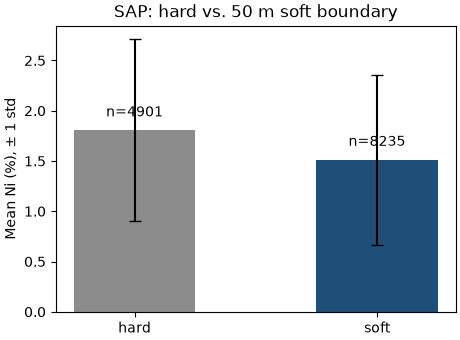
hard: n=4901, mean=1.81 % Ni, variance=0.822
soft: n=8235, mean=1.51 % Ni, variance=0.714
every LIM sample sits within 50 m, straight-line, of some SAP sample. the holes are on a 50 m mesh (25 m infill),
so this isotropic buffer folds in the whole of LIM, and the soft row of SAP becomes the pooled statistics of both
horizons. that is the most that opening the boundary at 50 m could do: the mean of SAP falls from 1.81 % Ni (hard,
its own 4901 samples) to 1.51 % once all 3334 LIM samples join it. the variance falls too, from 0.82 to 0.71, though
the CV rises since the mean moves further than the spread. the anisotropic ellipsoid of the search is far tighter,
reaching only about 5 m up or down at 50 m across, so the shift that kriging sees is local and much smaller:
soft boundaries found 1.55 % against 1.28 % held out in the last
meter of SAP hardened, and 1.34 % opened one way. soft_boundary bounds the dilution that a distance-only buffer
would risk, which is why the search measures distance in the fitted ellipsoid.
fig, ax = plt.subplots(figsize=(4.6, 3.4), layout="constrained")
kinds = list(stats["kind"])
ax.bar(kinds, stats["mean"], yerr=stats["std"], color=[GRAY, ACCENT], capsize=4, width=0.5)
for i, (n, m) in enumerate(zip(stats["n"], stats["mean"], strict=True)):
    ax.annotate(f"n={n:.0f}", (i, m), textcoords="offset points", xytext=(0, 10), ha="center")
ax.set(ylabel="Mean Ni (%), ± 1 std", title="SAP: hard vs. 50 m soft boundary")
save(fig, "soft_boundary")
Total running time of the script: ( 0 minutes 0.097 seconds)
Download Python source code: example_03_08.py