variogram sets¶

experimental_variograms computes every direct and cross variogram of several variables in one call. the set it returns is indexed by variable pair; Coregionalization.fit takes it as it is, and bt.plot.variograms draws it as a matrix of panels. on a regular grid the call finds pairs by shifting cell indices instead of comparing every two samples, so variograms of exhaustive grids and simulated realizations are cheap.

import sys
from pathlib import Path

HERE = Path(__file__).parent if "__file__" in globals() else Path.cwd()
sys.path.insert(0, str(HERE.parents[1]))

import boitata as bt
import numpy as np
from common import save

train = bt.datasets.jura()["prediction"]
metals = ["Cd", "Co", "Cr", "Cu", "Ni", "Pb", "Zn"]

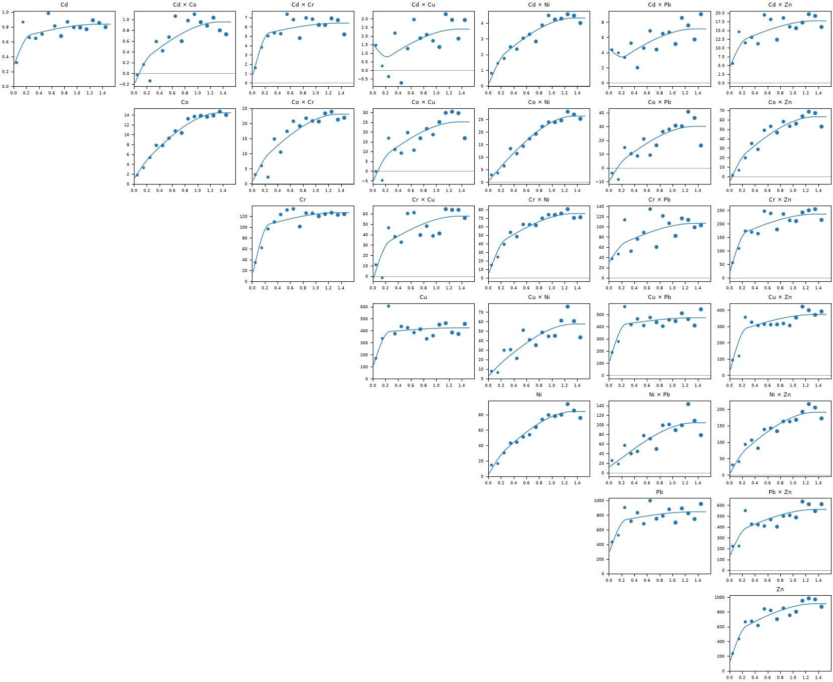
jura has seven metals at 259 soil samples, in km. one call gives the 7 direct and 21 cross variograms. vs[i, j] and vs[j, i] are the same cross variogram, and you can name variables by column.

vs = bt.experimental_variograms(train, metals, 0.1, 1.5)
print(vs)
print(f"Cd × Zn: {len(vs['Cd', 'Zn'].lags)} lags, {int(vs['Cd', 'Zn'].counts.sum()):,} pairs")

Out:

VariogramSet(7 variables, omnidirectional)
Cd × Zn: 15 lags, 11,376 pairs

the linear model of coregionalization fits all 28 at once. each structure has a 7 × 7 sill matrix, kept positive semi-definite, so the model is valid for cokriging any subset of the metals. its total sill matrix gives correlations between the metals close to those of the samples:

lmc = bt.Coregionalization.fit(vs, ["spherical", "spherical"])
for name, matrix in [("nugget", lmc.nugget)] + [(f"{m} {a:.2f} km", s) for m, a, s in lmc.structures]:
    print(f"{name:18} smallest eigenvalue {np.linalg.eigvalsh(matrix)[0]:.2g}")
sill = lmc.nugget + sum(s for _, _, s in lmc.structures)
model_corr = sill / np.sqrt(np.outer(np.diag(sill), np.diag(sill)))
sample_corr = bt.correlation(train, columns=metals)
upper = np.triu_indices(len(metals), 1)
print(f"largest |model - sample| correlation: {np.abs(model_corr - sample_corr)[upper].max():.2f}")

Out:

nugget             smallest eigenvalue -5.8e-14
spherical 0.27 km  smallest eigenvalue -6.8e-14
spherical 1.36 km  smallest eigenvalue -6.5e-14
largest |model - sample| correlation: 0.10

the diagonal holds the direct variograms and the panels above it the cross variograms, each with the fitted model. Co and Ni gain most of their sill over the long structure, Cu and Pb over the short one, and each cross variogram mixes the two in its own proportions.

fig, axes = bt.plot.variograms(vs, model=lmc)
for ax in axes.flat:
    ax.title.set_fontsize(8)
    ax.tick_params(labelsize=6)
    ax.xaxis.label.set_visible(False)
    ax.yaxis.label.set_visible(False)
save(fig, "jura")

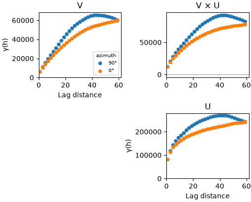
Cd, Cd × Co, Cd × Cr, Cd × Cu, Cd × Ni, Cd × Pb, Cd × Zn, Co, Co × Cr, Co × Cu, Co × Ni, Co × Pb, Co × Zn, Cr, Cr × Cu, Cr × Ni, Cr × Pb, Cr × Zn, Cu, Cu × Ni, Cu × Pb, Cu × Zn, Ni, Ni × Pb, Ni × Zn, Pb, Pb × Zn, Zn

the walker lake exhaustive grid holds V and U at all 78 000 cells of a 260 × 300 m grid. given a BlockModel, all pairs one cell offset apart share a separation, so the call bins each offset once and gathers its pairs by index shifts. with a half-degree tolerance only the offsets along the rows and columns remain: 30 lags per direction, each one pass over the cells.

table = bt.datasets.walker_lake_exhaustive()
grid = bt.BlockModel((0.5, 0.5), (1.0, 1.0), (260, 300), attributes={"V": table["V"], "U": table["U"]})
axes_set = bt.experimental_variograms(
    grid, ["V", "U"], 2.0, 60.0, directions=[(90.0, 0.0), (0.0, 0.0)], tolerance=0.5
)
east, north = axes_set["V", "V"]
print(f"V along x: {int(east.counts.sum()):,} pairs; along y: {int(north.counts.sum()):,} pairs")

Out:

V along x: 4,131,000 pairs; along y: 4,204,200 pairs

on a 60 × 60 m corner, small enough for the search over cell centers, the index shifts find the same pairs and the same estimates up to round-off:

corner = bt.BlockModel((0.5, 0.5), (1.0, 1.0), (60, 60))
rows = (np.arange(60)[:, None] * 260 + np.arange(60)).ravel()
v = table["V"][rows]
by_shift = bt.experimental_variogram(corner, v, 2.0, 30.0)
by_search = bt.experimental_variogram(corner, v, 2.0, 30.0, method="pairs")
print(f"same pair counts: {np.array_equal(by_shift.counts, by_search.counts)}")
print(f"largest relative difference in γ: {np.max(np.abs(by_shift.gammas / by_search.gammas - 1)):.1e}")

Out:

same pair counts: True
largest relative difference in γ: 1.1e-15

V is more continuous north to south than east to west, and U follows it. the same call on a simulated realization checks it against the variogram model it was drawn from.

fig, axes = bt.plot.variograms(axes_set)
save(fig, "walker_lake")