domain cleanup¶

a rock-type model estimated or simulated block by block carries specks: single blocks or small clusters of one rock inside another, too small to mine or to model apart. remove_small_units finds the connected units of each rock and gives each unit below a minimum volume to the rock around it. contact_distance then measures how far each block is from a contact, and buffer_domains labels the blocks within a given distance of one: the transition zone where a soft boundary (soft boundaries) lets samples cross.

import sys
import warnings
from pathlib import Path

HERE = Path(__file__).parent if "__file__" in globals() else Path.cwd()
sys.path.insert(0, str(HERE.parents[1]))
warnings.filterwarnings("ignore", ".*locations hold several samples")

import boitata as bt
import matplotlib.pyplot as plt
import numpy as np
from common import save

a speckled rock model¶

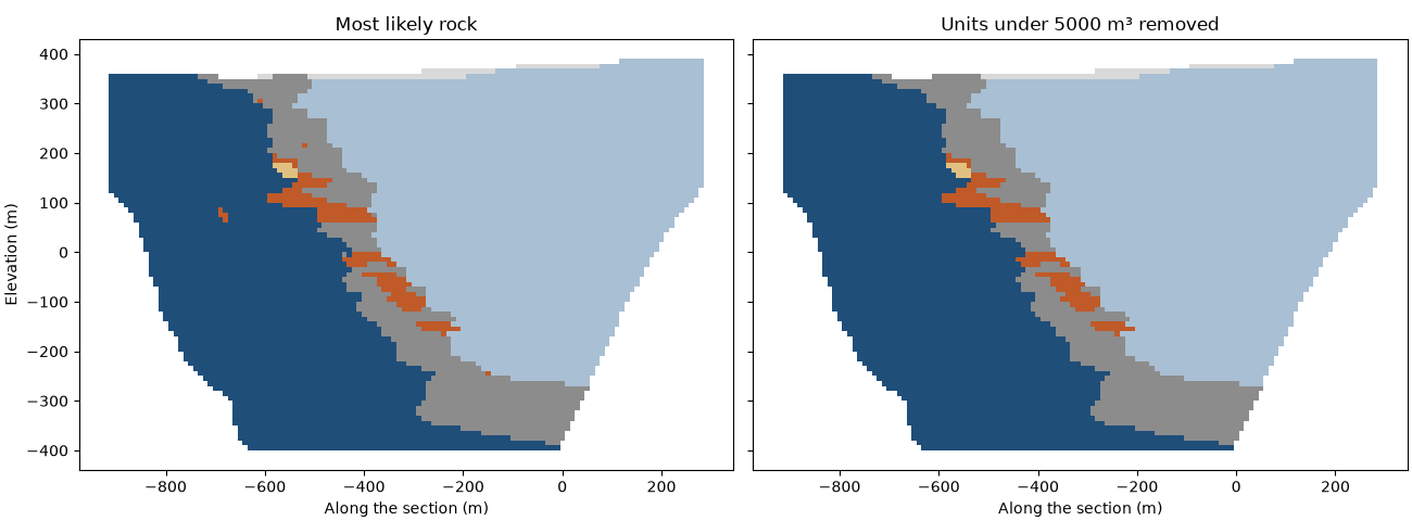
the most likely rock from categorical indicator kriging of the logged rock types of the stacked sulphide lenses on a vertical section across strike, cells of 10 m, one cell thick. cells the search left unestimated are dropped. choosing the most likely rock cell by cell leaves specks, such as the sulphide cells inside the footwall volcanics on the left.

data = bt.datasets.stacked_sulphide_lenses()
drillholes = bt.Drillholes.from_tables(data, intervals="lithology")
composites = drillholes.composite(5.0, [], categories=["LITH"])
scheme = bt.Categories(
    ["OB", "HWS", "VCL", "SUL", "FWV"],
    mapping={"MS": "SUL", "SMS": "SUL", "STR": "SUL"},
    other="DYK",
    colors=["#d9d9d9", "#a9bfd3", "#8c8c8c", "#c05a28", "#1f4e79", "#e0c080"],
)
weights = bt.cell_declustering(composites, scheme.encode(composites["LITH"]), cell_size=50.0).weights
layers = (23.0, 55.0, 0.0)
variograms = [
    bt.Variogram([("spherical", 0.9, 400.0)], nugget=0.1, rotation=(0.0, 0.0, 0.0), ratios=(1.0, 0.05)),
    bt.Variogram([("spherical", 0.9, 500.0)], nugget=0.1, rotation=layers, ratios=(0.8, 0.2)),
    bt.Variogram([("spherical", 0.85, 400.0)], nugget=0.15, rotation=layers, ratios=(0.8, 0.2)),
    bt.Variogram([("spherical", 0.8, 150.0)], nugget=0.2, rotation=layers, ratios=(0.8, 0.25)),
    bt.Variogram([("spherical", 0.9, 500.0)], nugget=0.1, rotation=layers, ratios=(0.8, 0.2)),
    bt.Variogram([("spherical", 0.7, 40.0)], nugget=0.3),
]
passes = [
    bt.Search(150.0, max_samples=24, max_per_hole=6, rotation=layers, ratios=(1.0, 0.4)),
    bt.Search(300.0, max_samples=24, rotation=layers, ratios=(1.0, 0.4)),
]
cik = bt.CategoricalIndicatorKriging(variograms, passes, scheme=scheme)
cik.fit(composites, "LITH", weights=weights, holes="HOLE_ID")

center = np.array([12350.0, 29900.0, 0.0])
across = np.array([np.sin(np.radians(113.0)), np.cos(np.radians(113.0)), 0.0])
along = np.array([np.sin(np.radians(23.0)), np.cos(np.radians(23.0)), 0.0])
origin = center - 600.0 * across - 5.0 * along + [0.0, 0.0, -400.0]
section = bt.BlockModel(origin, (10.0, 10.0, 10.0), (120, 1, 80), rotation=(23.0, 0.0, 0.0))
topography = data["topography"]
section = section.filter(section.z < topography.sample(section.coords[:, :2], "Z"))
section = section.with_columns({"rock": cik.predict(section).most_likely}).drop_null("rock")
print(f"{len(section)} cells of {section.volumes[0]:.0f} m³")

Out:

7645 cells of 1000 m³

removing the specks¶

a unit is a set of blocks of one rock joined through shared faces (connectivity=6, here the four neighbors in the section) or also through edges and corners (connectivity=26). units go smallest first. each goes to the rock with the most volume among the blocks touching it and merges with the units of that rock. a unit stays below the minimum only when it has no neighbor to join, walled in by absent cells or, with domains=, by other domains; here there are none. the minimum is five cells, 5000 m³. the total volume stays the same and only its split changes.

section = section.with_columns({"clean": bt.remove_small_units(section, "rock", min_volume=5000.0)})
volume = section.volumes
changed = section["rock"] != section["clean"]
print(f"{changed.sum()} cells change rock")
print(f"{'':<5}{'before (m³)':>13}{'after (m³)':>12}")
for code, name in enumerate(scheme.names):
    before, after = volume[section["rock"] == code].sum(), volume[section["clean"] == code].sum()
    print(f"{name:<5}{before:13.0f}{after:12.0f}")
print(f"total volume kept: {volume[section['rock'] >= 0].sum() == volume[section['clean'] >= 0].sum()}")

Out:

12 cells change rock
       before (m³)  after (m³)
OB           67000       64000
HWS        3549000     3551000
VCL         929000      932000
SUL         188000      181000
FWV        2901000     2906000
DYK          11000       11000
total volume kept: True

fig, axes = plt.subplots(1, 2, figsize=(13, 4.8), layout="constrained", sharey=True)
for ax, column, title in zip(axes, ["rock", "clean"], ["Most likely rock", "Units under 5000 m³ removed"]):
    bt.plot.section(section, column, axis="y", index=0, scheme=scheme, colorbar=False, ax=ax)
    ax.set_title(title)
    ax.set_xlabel("Along the section (m)")
axes[0].set_ylabel("Elevation (m)")
axes[1].set_ylabel("")
save(fig, "cleanup")

Most likely rock, Units under 5000 m³ removed

distance to the contacts¶

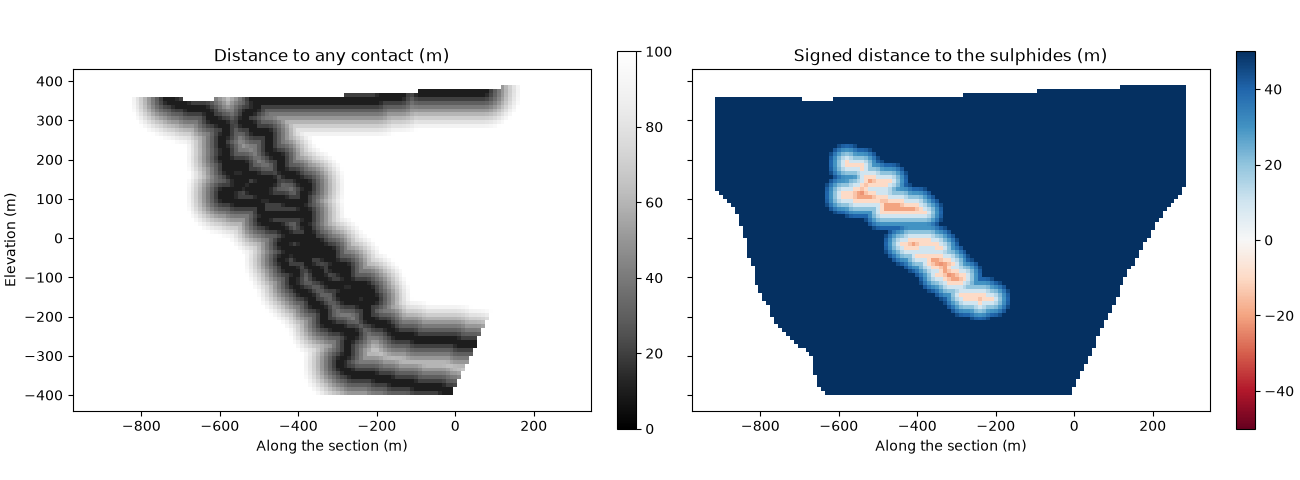
contact_distance gives each block the distance from its centroid to the nearest block centroid of another rock, or with target=, of that rock. blocks of the target get the distance to the nearest block outside it, negative by default, so the field is signed across the target's contact. distances are exact in any layout and rotation, and the two blocks either side of a contact get the same distance.

to_sulphide = bt.contact_distance(section, "clean", target=scheme.names.index("SUL"))
to_any = bt.contact_distance(section, "clean")
fig, axes = plt.subplots(1, 2, figsize=(13, 4.8), layout="constrained", sharey=True)
bt.plot.section(section, to_any, axis="y", index=0, vmin=0.0, vmax=100.0, cmap="Greys_r", ax=axes[0])
axes[0].set_title("Distance to any contact (m)")
bt.plot.section(section, to_sulphide, axis="y", index=0, vmin=-50.0, vmax=50.0, cmap="RdBu", ax=axes[1])
axes[1].set_title("Signed distance to the sulphides (m)")
for ax in axes:
    ax.set_xlabel("Along the section (m)")
axes[0].set_ylabel("Elevation (m)")
axes[1].set_ylabel("")
save(fig, "distances")

Distance to any contact (m), Signed distance to the sulphides (m)

contact buffers¶

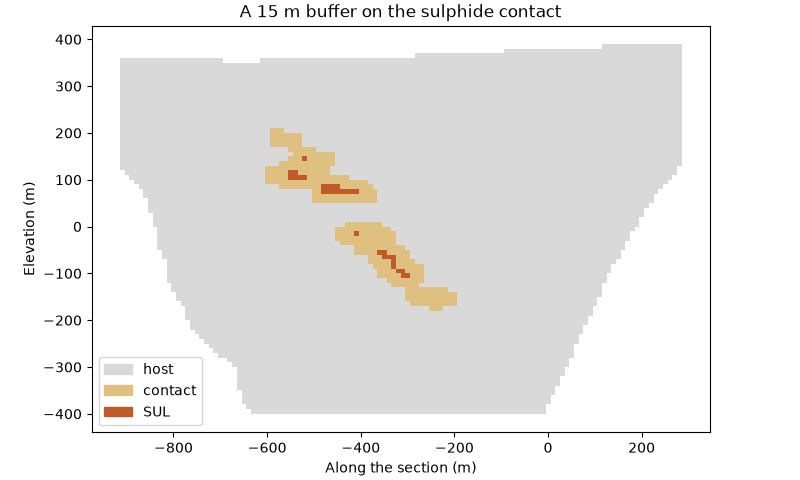
buffer_domains relabels each block within distance of a contact as label, here the blocks within 15 m of the sulphide contact: those sharing a face or an edge with a block across it. both sides of a contact read the same distance, so the buffer takes one ring of blocks inside the sulphides and one outside. the host ring is the longer one, as it wraps the lenses, and the thinnest lenses fall inside the buffer whole. you can treat the buffer as a domain of its own for statistics, or as the zone in which a soft boundary shares samples between the sulphides and their host.

sulphide = np.where(section["clean"] == scheme.names.index("SUL"), "SUL", "host")
zone = bt.buffer_domains(section, sulphide, distance=15.0, target="SUL")
zones = bt.Categories(["host", "contact", "SUL"], colors=["#d9d9d9", "#e0c080", "#c05a28"])
section = section.with_columns({"zone": zones.encode(zone)})
for name in ("SUL", "host"):
    print(f"{name} cells in the buffer: {np.sum((zone == 'contact') & (sulphide == name))}")

fig, ax = plt.subplots(figsize=(8, 4.8), layout="constrained")
bt.plot.section(section, "zone", axis="y", index=0, scheme=zones, colorbar=False, ax=ax)
bt.plot.category_legend(zones, ax=ax, loc="lower left")
ax.set_title("A 15 m buffer on the sulphide contact")
ax.set_xlabel("Along the section (m)")
ax.set_ylabel("Elevation (m)")
save(fig, "buffer")

A 15 m buffer on the sulphide contact

Out:

SUL cells in the buffer: 150
host cells in the buffer: 199

Total running time of the script: ( 0 minutes 1.967 seconds)

Download Python source code: example_02_14.py

Download Jupyter notebook: example_02_14.ipynb

Gallery generated by mkdocs-gallery