Note
Click here to download the full example code
seismic volumes
bt.read_segy reads a post-stack SEG-Y cube into a 3D BlockModel, one trace per column of cells, and
bt.write_segy writes one back. seismic covers the whole volume where wells are few, so it serves as the secondary
variable that steers image quilting between them.
import sys
import tempfile
from pathlib import Path

HERE = Path(__file__).parent if "__file__" in globals() else Path.cwd()
sys.path.insert(0, str(HERE.parents[1]))
import boitata as bt
import matplotlib.pyplot as plt
import numpy as np
from common import HIGHLIGHT, INK, save
from matplotlib.colors import ListedColormap

cube = bt.read_segy(bt.datasets.fetch("oil-gas/3d/f3-seismic/seismic.sgy"))
nx, ny, nz = cube.count
print(f"{nx} inlines x {ny} crosslines x {nz} samples")
print(
    f"cells {cube.size[0]:.1f} x {cube.size[1]:.1f} m x {cube.size[2]:.0f} ms, azimuth {cube.rotation[0]:.1f}°"
)
print(f"first sample at {-(cube.origin[2] + (nz - 0.5) * cube.size[2]):.0f} ms, CRS {cube.crs}")
Out:
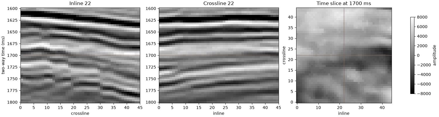
45 inlines x 45 crosslines x 51 samples
cells 25.0 x 25.0 m x 4 ms, azimuth 88.4°
first sample at 1600 ms, CRS None
inline and crossline numbers come from trace-header bytes 189 and 193 and the CDP coordinates from bytes 181 and
185, the SEG-Y revision 1 places; inline_byte, crossline_byte, x_byte and y_byte move them for files that
put them elsewhere. the file states no CRS, so the cube has none; bt.datasets.f3_seismic() sets it. z is minus the
two-way time, so a time slice is a z layer, and the first sample is the top cell.
amplitude = cube.grid("amplitude")[::-1]  # row 0 at the first sample
times = (1598, 1598 + 4 * nz)
style = {"cmap": "gray", "vmin": -8000, "vmax": 8000, "interpolation": "nearest"}
fig, axes = plt.subplots(1, 3, figsize=(15, 4), layout="constrained", width_ratios=[1, 1, 0.9])
im = axes[0].imshow(amplitude[:, :, 22], extent=(0, ny, times[1], times[0]), aspect="auto", **style)
axes[0].set(title="Inline 22", xlabel="crossline", ylabel="two-way time (ms)")
axes[1].imshow(amplitude[:, 22, :], extent=(0, nx, times[1], times[0]), aspect="auto", **style)
axes[1].set(title="Crossline 22", xlabel="inline")
axes[2].imshow(amplitude[25], origin="lower", **style)
axes[2].set(title=f"Time slice at {1600 + 4 * 25} ms", xlabel="inline", ylabel="crossline")
for ax in axes[:2]:
    ax.axhline(1600 + 4 * 25, color=HIGHLIGHT, lw=0.8)
axes[2].axvline(22, color=HIGHLIGHT, lw=0.8)
axes[2].axhline(22, color=HIGHLIGHT, lw=0.8)
fig.colorbar(im, ax=axes, shrink=0.8, label="amplitude")
save(fig, "cube")
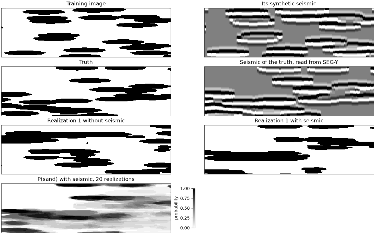
quilting with seismic needs a training image that carries both facies and the seismic they would produce: here a section 200 traces wide and 80 samples deep, of sand lenses 50 by 8 cells in shale, and its synthetic seismic. sand has a lower acoustic impedance, each change of impedance down a trace makes a reflection, and a ricker wavelet blurs the reflections into amplitude. the truth is another section drawn the same way, and you know only its seismic.
width, depth = 200, 80
section = bt.BlockModel((0, 0), (1, 1), (width, depth))
lens = {"shape": "ellipsoid", "code": 1, "proportion": 0.3, "radii": (25, 4), "azimuth": 90}


def synthetic_seismic(facies):
    impedance = np.where(facies.reshape(depth, width) == 1, 5.0, 7.0)
    reflectivity = np.zeros_like(impedance)
    reflectivity[1:] = np.diff(impedance, axis=0) / (impedance[1:] + impedance[:-1])
    t = np.pi * 0.08 * np.arange(-8, 9)
    ricker = (1 - 2 * t**2) * np.exp(-(t**2))
    return np.apply_along_axis(np.convolve, 0, reflectivity, ricker, "same")


ti = bt.object_training_image(section, [lens], seed=1)
ti = ti.with_columns({"seismic": synthetic_seismic(ti["facies"]).ravel()})
truth = bt.object_training_image(section, [lens], seed=2).grid("facies")[0]
the truth's seismic arrives as a SEG-Y file. write_segy takes a 3D model, one trace per (x, y) column: here one
crossline of 200 traces 12.5 m apart, sampled every 4 ms from 1600 ms. read back, it matches to float32.
survey = bt.BlockModel((0, 0, -1598 - 4 * depth), (12.5, 12.5, 4), (width, 1, depth))
survey = survey.with_columns({"seismic": synthetic_seismic(truth)[::-1].ravel()})  # bottom layer first
with tempfile.TemporaryDirectory() as folder:
    path = Path(folder) / "truth.sgy"
    bt.write_segy(path, survey, "seismic")
    back = bt.read_segy(path, column="seismic")
print(f"read back {back.count}, largest difference {np.abs(back['seismic'] - survey['seismic']).max():.1e}")
secondary = back.grid("seismic")[::-1].ravel()
Out:
read back [200, 1, 80], largest difference 1.5e-08
twenty realizations of the truth without and with the seismic. with secondary, quilting also chooses a patch by
how well the image's seismic under it matches the target's: secondary_weight times the mean squared difference
over the squared range, beside its overlap. the score is the mean probability each realization gives the true
facies of a cell: 0.58 for random draws at the image's proportions.
def agreement(summary):
    p_sand = summary.probabilities[:, 1]
    return np.where(truth.ravel() == 1, p_sand, 1 - p_sand).mean()


blind = bt.ImageQuilting(ti, "facies", patch_size=20).simulate(section, n=20, seed=1, keep=[0])
steered = bt.ImageQuilting(ti, "facies", patch_size=20, secondary="seismic").simulate(
    section, n=20, seed=1, keep=[0], secondary=secondary
)
for name, summary in (("without seismic", blind), ("with seismic", steered)):
    print(
        f"{name}: sand {summary.proportions[:, 1].mean():.1%}, agreement with the truth {agreement(summary):.2f}"
    )
Out:
without seismic: sand 33.3%, agreement with the truth 0.56
with seismic: sand 27.1%, agreement with the truth 0.74
the seismic places the lenses. nearly all realizations find an isolated lens. where lenses stack a few samples apart, their reflections overlap, several arrangements of patches fit the same seismic, and the probability of sand stays gray.
codes = ListedColormap(["white", "black"])
panels = (
    (ti["facies"], "Training image", codes, None),
    (ti["seismic"], "Its synthetic seismic", "gray", 0.12),
    (truth, "Truth", codes, None),
    (secondary, "Seismic of the truth, read from SEG-Y", "gray", 0.12),
    (blind.realizations[0], "Realization 1 without seismic", codes, None),
    (steered.realizations[0], "Realization 1 with seismic", codes, None),
    (steered.probabilities[:, 1], "P(sand) with seismic, 20 realizations", "gray_r", None),
)
fig, axes = plt.subplots(4, 2, figsize=(12, 7.5), layout="constrained")
for ax, (values, title, cmap, clip) in zip(axes.flat, panels):
    limits = {"vmin": -clip, "vmax": clip} if clip else {"vmin": 0, "vmax": 1}
    im = ax.imshow(
        np.reshape(values, (depth, width)), cmap=cmap, interpolation="nearest", aspect="auto", **limits
    )
    ax.set(title=title, xticks=[], yticks=[])
    for side in ax.spines.values():
        side.set(visible=True, color=INK, lw=0.6)
axes[3, 1].axis("off")
fig.colorbar(im, ax=axes[3, 1], location="left", shrink=0.8, label="probability")
save(fig, "quilting")
hard data and soft probabilities combine with the secondary variable, each with its own weight; see image quilting. a 3D training image and target work the same way, with graph cuts joining the patches instead of boundary cuts.
Total running time of the script: ( 0 minutes 1.015 seconds)
Download Python source code: example_13_10.py