spatial bootstrap¶

a declustered mean is one number from a few hundred holes. how far off could it be? the classical bootstrap resamples the holes independently and answers σ/√n, but neighboring holes carry much the same information, so the true uncertainty is larger. bt.spatial_bootstrap resamples with the spatial correlation. each realization draws unconditional gaussian values at the holes with the normal-score variogram, turns them into ranks, and reads the ranks through the declustered distribution of the data. nearby holes then get similar draws, and the resampled mean spreads as far as the correlation allows.

import sys
from pathlib import Path

HERE = Path(__file__).parent if "__file__" in globals() else Path.cwd()
sys.path.insert(0, str(HERE.parents[1]))

import boitata as bt
import matplotlib.pyplot as plt
import numpy as np
from common import ACCENT, GRAY, HIGHLIGHT, INK, LIGHT, save

data = bt.datasets.coal_seam_thickness()
holes, grid = data["boreholes"], data["grid"]
thickness = holes["THICKNESS_M"]
xy = holes.coords[:, :2]
weights = bt.cell_declustering(holes, "THICKNESS_M", sizes=np.arange(100.0, 3100.0, 100.0)).weights
stats = bt.describe(thickness, weights=weights)
mean, sd = stats["mean"], stats["std"]
print(f"{len(holes)} holes, declustered mean {mean:.2f} m, standard deviation {sd:.2f} m")

Out:

295 holes, declustered mean 1.91 m, standard deviation 0.83 m

the resampling runs on the variogram of the normal scores. thicknesses are logged to the centimeter and many repeat, so bt.despike breaks the ties first; the fitted variogram is then rescaled to a unit sill.

untied = bt.despike(holes, "THICKNESS_M", seed=0)
scores = bt.NormalScore().fit_transform(untied, weights=weights)
fitted = bt.Variogram.fit(bt.experimental_variogram(xy, scores, 250.0, 6000.0), "spherical")
structure = fitted.structures[0]
variogram = fitted.standardized()
print(variogram)

nugget = bt.Variogram([], nugget=1.0)
independent = bt.spatial_bootstrap(holes, "THICKNESS_M", nugget, weights=weights, n=1000)
spatial = bt.spatial_bootstrap(holes, "THICKNESS_M", variogram, weights=weights, n=1000)
for name, table in (("independent", independent), ("spatial", spatial)):
    print(f"{name:>11}: standard deviation of the mean {np.std(table['mean']):.3f} m")
print(f"        σ/√n: {sd / np.sqrt(len(holes)):.3f} m")

Out:

Variogram(nugget=0.1952192065899283, structures=[Structure("spherical", sill=0.8047807934100717, range=2960.08750426967)], rotation=(0.0, 0.0, 0.0), ratios=(1.0, 1.0))
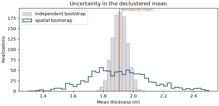
independent: standard deviation of the mean 0.048 m
    spatial: standard deviation of the mean 0.206 m
        σ/√n: 0.048 m

a pure-nugget variogram makes every draw independent, which gives the classical bootstrap: its spread matches σ/√n. with the fitted variogram, whose range is about 3 km over an 11 × 7 km lease, the spread is four times wider:

bins = np.linspace(1.3, 2.5, 49)
fig, ax = plt.subplots(figsize=(7, 3.4), layout="constrained")
ax.hist(independent["mean"], bins, color=LIGHT, edgecolor=GRAY, lw=0.5, label="independent bootstrap")
ax.hist(spatial["mean"], bins, histtype="step", color=ACCENT, lw=1.6, label="spatial bootstrap")
ax.axvline(mean, color=HIGHLIGHT, lw=1.2)
ax.text(mean, ax.get_ylim()[1], " declustered mean", color=HIGHLIGHT, va="top", fontsize=8)
ax.set(xlabel="Mean thickness (m)", ylabel="Realizations", title="Uncertainty in the declustered mean")
ax.legend(loc="upper left")
save(fig, "means")

Uncertainty in the declustered mean

range and effective number of holes¶

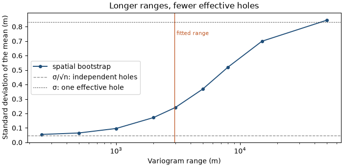
the spread grows with the range. as an effective number of independent holes, (σ / spread)², the 295 holes count as about a dozen at the fitted range of 3 km, and as one once the range spans the whole lease.

ranges = np.array([250.0, 500.0, 1000.0, 2000.0, 3000.0, 5000.0, 8000.0, 15000.0, 50000.0])
spreads = np.array(
    [
        np.std(
            bt.spatial_bootstrap(
                holes, "THICKNESS_M", bt.Variogram([("spherical", 1.0, r)]), weights=weights, n=400
            )["mean"]
        )
        for r in ranges
    ]
)
for r, s in zip(ranges, spreads):
    print(f"range {r:>7.0f} m: spread {s:.3f} m, effective holes {(sd / s) ** 2:.0f}")

fig, ax = plt.subplots(figsize=(7, 3.4), layout="constrained")
ax.semilogx(ranges, spreads, "o-", color=ACCENT, lw=1.4, ms=4, label="spatial bootstrap")
ax.axhline(sd / np.sqrt(len(holes)), color=GRAY, ls="--", lw=1, label="σ/√n: independent holes")
ax.axhline(sd, color=INK, ls=":", lw=1, label="σ: one effective hole")
ax.axvline(structure.range, color=HIGHLIGHT, lw=1)
ax.text(structure.range, sd * 0.93, " fitted range", color=HIGHLIGHT, va="top", fontsize=8)
ax.set(
    xlabel="Variogram range (m)",
    ylabel="Standard deviation of the mean (m)",
    title="Longer ranges, fewer effective holes",
    ylim=(0, sd * 1.08),
)
ax.legend(loc="center left")
save(fig, "ranges")

Longer ranges, fewer effective holes

Out:

range     250 m: spread 0.055 m, effective holes 228
range     500 m: spread 0.065 m, effective holes 163
range    1000 m: spread 0.096 m, effective holes 75
range    2000 m: spread 0.172 m, effective holes 23
range    3000 m: spread 0.241 m, effective holes 12
range    5000 m: spread 0.369 m, effective holes 5
range    8000 m: spread 0.521 m, effective holes 3
range   15000 m: spread 0.699 m, effective holes 1
range   50000 m: spread 0.844 m, effective holes 1

tonnage uncertainty¶

the lease covers the cells flagged INSIDE; at 1.4 t/m³ each realization of the mean thickness gives a tonnage. the table also returns quantiles and proportions above cutoffs per realization, here the share of the seam thicker than 2 m, the minimum mining height.

area = np.sum(grid["INSIDE"] == 1) * 100.0 * 100.0
density = 1.4
for name, v in (("independent", nugget), ("spatial", variogram)):
    table = bt.spatial_bootstrap(holes, "THICKNESS_M", v, weights=weights, n=1000, cutoffs=[2.0])
    tonnes = table["mean"] * area * density / 1e6
    p10, p50, p90 = np.quantile(tonnes, [0.1, 0.5, 0.9])
    above = np.quantile(table["above 2"], [0.1, 0.9])
    print(
        f"{name:>11}: P10 {p10:.0f} Mt, P50 {p50:.0f} Mt, P90 {p90:.0f} Mt;"
        f" thicker than 2 m {above[0]:.0%} to {above[1]:.0%}"
    )

Out:

independent: P10 185 Mt, P50 191 Mt, P90 198 Mt; thicker than 2 m 34% to 41%
    spatial: P10 167 Mt, P50 190 Mt, P90 219 Mt; thicker than 2 m 25% to 50%

independent resampling promises the tonnage within a few percent; with the spatial correlation the P10 to P90 range is four times wider. that range is the uncertainty in the global mean from the holes alone, before any estimate or simulation. it sets a lower bound on what a resource can claim and tells you whether more holes would pay.

Total running time of the script: ( 0 minutes 0.287 seconds)

Download Python source code: example_03_12.py

Download Jupyter notebook: example_03_12.ipynb

Gallery generated by mkdocs-gallery