Note
Click here to download the full example code
statistics by domain
three stacked sulphide lenses, logged as massive (MS), semi-massive (SMS) and stringer (STR) sulphides in volcanic and sedimentary host rocks. do the lithologies differ enough to estimate them apart? statistics, box plots, cumulative distributions and Q-Q plots per lithology on 2 m composites.
import sys
from pathlib import Path

HERE = Path(__file__).parent if "__file__" in globals() else Path.cwd()
sys.path.insert(0, str(HERE.parents[1]))
import boitata as bt
import matplotlib.pyplot as plt
import numpy as np
from common import save

data = bt.datasets.stacked_sulphide_lenses()
intervals = bt.merge_intervals(data["assays"], data["lithology"])
holes = bt.Drillholes(data["collars"], data["surveys"], intervals)
composites = holes.composite(2.0, ["ZN_PCT", "CU_PCT"], domain="LITH")
print(f"{len(composites)} composites")
Out:
13602 composites
describe_by gives the count, moments and quantiles of a column per category, then over all values on the last row.
it skips missing grades, and weights= takes declustering weights
(declustering).
stats = bt.describe_by("ZN_PCT", "LITH", quantiles=[0.1, 0.5, 0.9], data=composites)
print(f"{'LITH':<6}{'n':>7}{'mean':>8}{'CV':>6}{'P10':>8}{'P50':>8}{'P90':>8}{'max':>8}")
for row in zip(*(stats[c] for c in ["category", "n", "mean", "cv", "P10", "P50", "P90", "max"]), strict=True):
    print(f"{row[0]:<6}{row[1]:>7.0f}{row[2]:>8.2f}{row[3]:>6.2f}" + "".join(f"{v:>8.2f}" for v in row[4:]))
Out:
LITH        n    mean    CV     P10     P50     P90     max
DYK        74    0.06  0.66    0.02    0.05    0.12    0.20
FWV      1599    0.06  0.68    0.02    0.05    0.10    0.49
HWS      1448    0.05  0.66    0.02    0.04    0.09    0.36
MS        627    8.94  0.55    3.67    7.96   15.25   37.06
SMS       652    3.44  0.61    1.38    2.98    5.86   15.36
STR       583    0.38  0.56    0.18    0.34    0.67    1.52
VCL      8619    0.05  0.67    0.02    0.04    0.09    0.35
all     13602    0.64  3.57    0.02    0.05    0.56   37.06
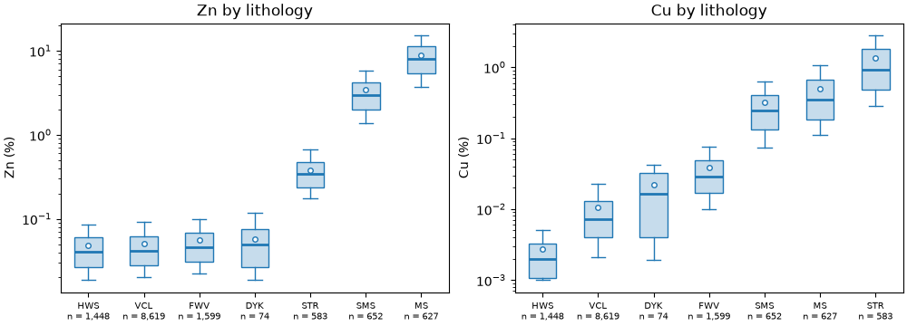
mean Zn falls from 8.94 % in MS to 3.44 % in SMS and 0.38 % in STR; the host rocks and the dyke hold 0.05 to 0.06 %. each lithology has a CV between 0.55 and 0.68, and all of them pooled reach 3.57: mixing populations makes that spread.
box plots show the same quantiles side by side, sorted by median. the box spans P25 to P75, the whiskers P10 to P90, and the dot marks the mean. Cu differs from Zn: it is richest in the stringer zone below the lenses.
lith = composites["LITH"]
fig, axes = plt.subplots(1, 2, figsize=(10, 3.6), layout="constrained")
for ax, grade in zip(axes, ["ZN_PCT", "CU_PCT"], strict=True):
    bt.plot.boxplot(grade, lith, sort=True, log=True, data=composites, ax=ax)
    ax.set(title=f"{grade.split('_')[0].title()} by lithology", ylabel=f"{grade.split('_')[0].title()} (%)")
    ax.tick_params(axis="x", labelsize=7)
save(fig, "boxplot")
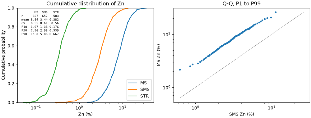
cumulative distributions compare whole distributions; stats=True lists the count, mean, CV and deciles of each curve
in the corner. the Q-Q plot pairs the quantiles of two lithologies, and points along the 1:1 line would mean the same
distribution. MS against SMS falls on a line parallel to it on log axes, a constant ratio: MS is SMS scaled up about
2.7 times, the same shape at a different grade.
zn = composites["ZN_PCT"]
sulphides = ["MS", "SMS", "STR"]
fig, (a, b) = plt.subplots(1, 2, figsize=(10, 3.8), layout="constrained")
bt.plot.cdf([zn[lith == k] for k in sulphides], labels=sulphides, log=True, stats=True, ax=a)
a.set(title="Cumulative distribution of Zn", xlabel="Zn (%)")
bt.plot.qq(zn[lith == "SMS"], zn[lith == "MS"], log=True, ax=b)
b.set(title="Q-Q, P1 to P99", xlabel="SMS Zn (%)", ylabel="MS Zn (%)")
save(fig, "distributions")
ratio = np.percentile(zn[lith == "MS"], [10, 50, 90]) / np.percentile(zn[lith == "SMS"], [10, 50, 90])
print("MS over SMS at P10, P50, P90:", ", ".join(f"{r:.1f}" for r in ratio))
Out:
MS over SMS at P10, P50, P90: 2.7, 2.7, 2.6
Total running time of the script: ( 0 minutes 0.668 seconds)
Download Python source code: example_03_02.py