kriging diagnostics¶

block kriging of walker lake V on 10 × 10 m blocks with diagnostics=True: kriging efficiency and slope of regression per block, then the neighborhood behind each estimate. the exhaustive grid checks what they predict.

import sys
from pathlib import Path

HERE = Path(__file__).parent if "__file__" in globals() else Path.cwd()
sys.path.insert(0, str(HERE.parents[1]))

import boitata as bt
import matplotlib.pyplot as plt
import numpy as np
from common import GRAY, map_axes, save

samples = bt.datasets.walker_lake()
truth = bt.datasets.walker_lake_exhaustive()["V"].reshape(300, 260)
xy, v = samples.coords, samples["V"]
azimuths = np.arange(0, 180, 22.5)
directional = [bt.experimental_variogram(xy, v, 10.0, 120.0, azimuth=a) for a in azimuths]
model = bt.Variogram.fit_directional(
    directional, [(a, 0) for a in azimuths], ["spherical", "spherical"], weighting="count/gamma"
)

blocks = bt.BlockModel(origin=(0.5, 0.5), size=(10, 10), count=(26, 30))
search = bt.Search(radius=80, max_samples=24, min_samples=4, rotation=model.rotation, ratios=(0.5, 1.0))
kriging = bt.BlockKriging(model, search, size=(10, 10), discretization=(5, 5, 1)).fit(xy, v)
d = kriging.predict(blocks, diagnostics=True)
true_blocks = truth.reshape(30, 10, 26, 10).mean(axis=(1, 3)).ravel()
extent = (0.5, 260.5, 0.5, 300.5)

efficiency and slope¶

kriging efficiency compares the block variance with the kriging variance: 1 for a block known without error, 0 or less for one no better known than the global mean. the slope of regression of true on estimated grades is 1 when estimates are conditionally unbiased; below 1, high estimates overstate and low ones understate the truth. both fall away from the samples:

fig, axes = plt.subplots(1, 2, figsize=(9, 4.6), layout="constrained")
for ax, key, title in (
    (axes[0], "efficiency", "Kriging efficiency"),
    (axes[1], "slope", "Slope of regression"),
):
    im = ax.imshow(blocks.grid(d[key])[0], origin="lower", extent=extent, vmin=0, vmax=1)
    ax.scatter(samples.x, samples.y, s=2, color=GRAY, linewidths=0)
    map_axes(ax, title)
fig.colorbar(im, ax=axes, shrink=0.8)
save(fig, "diagnostics")

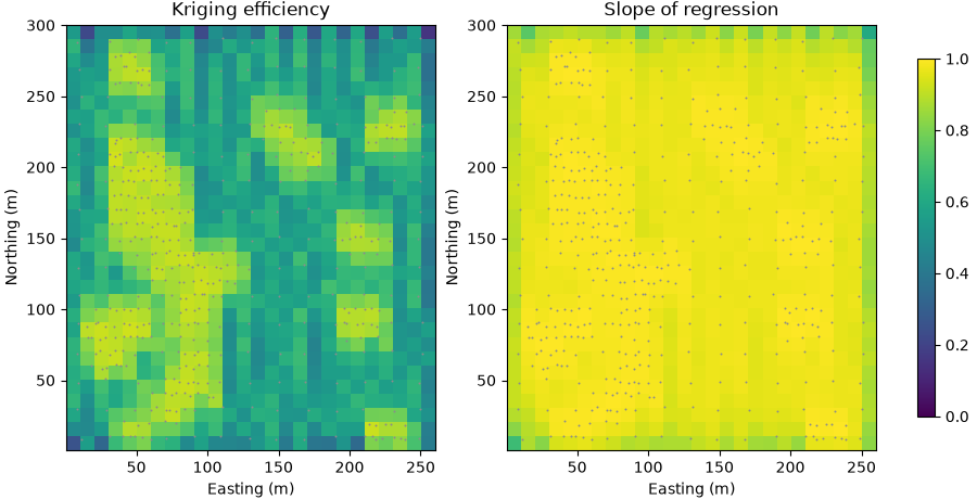
Kriging efficiency, Slope of regression

the truth checks both. over all blocks, the regression of true on estimated block grades has a slope close to the mean predicted slope. blocks with efficiency of 0.7 or more sit closer to the truth; below 0.7, efficiency separates them poorly, one reason classification also uses sample spacing (classification).

observed = np.polyfit(d["value"], true_blocks, 1)[0]
print(f"slope of regression: predicted mean {d['slope'].mean():.2f}, observed {observed:.2f}")
groups = np.digitize(d["efficiency"], [0.5, 0.7])
for g, label in enumerate(("efficiency < 0.5", "0.5 to 0.7", ">= 0.7")):
    k = groups == g
    c = bt.compare(d["value"][k], true_blocks[k])
    print(
        f"{label:>16}: {k.sum():3d} blocks, RMSE {c['rmse']:5.1f} ppm, correlation with truth {c['correlation']:.2f}"
    )

Out:

slope of regression: predicted mean 0.96, observed 1.02
efficiency < 0.5:  98 blocks, RMSE  95.7 ppm, correlation with truth 0.77
      0.5 to 0.7: 423 blocks, RMSE 110.0 ppm, correlation with truth 0.70
          >= 0.7: 259 blocks, RMSE  84.0 ppm, correlation with truth 0.93

neighborhood¶

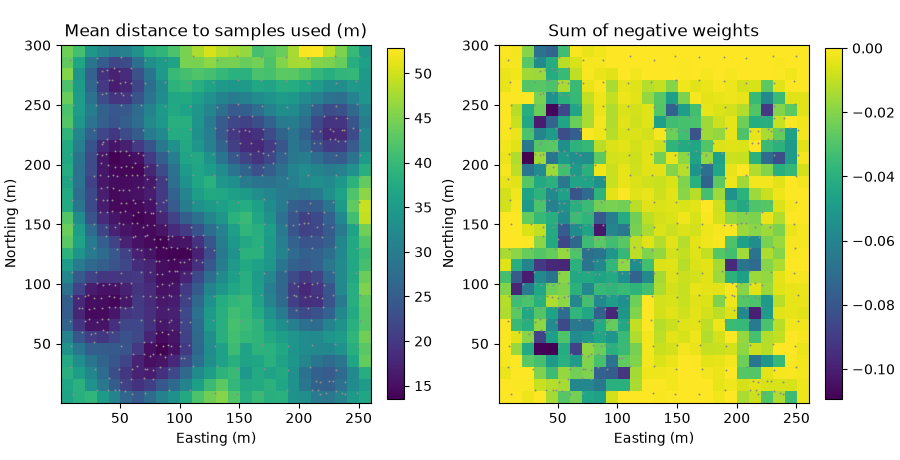
the other diagnostics explain why a block is weak. mean_distance is the mean distance to the samples used, and max_samples_reached flags searches that stopped at 24 samples before the ellipse ran out: those blocks sit in denser data and have the higher slope. negative_weight_sum adds the weights below zero, which samples screened by closer ones receive. lagrange (the lagrange multiplier) and n_holes (distinct drill holes used; each walker lake sample is its own) complete the set.

full = d["max_samples_reached"] == 1
for label, k in (("full search", full), ("ellipse ran out", ~full)):
    print(
        f"{label:>15}: {k.mean():4.0%} of blocks, mean distance {d['mean_distance'][k].mean():4.1f} m, "
        f"mean slope {d['slope'][k].mean():.2f}"
    )
groups = np.digitize(d["negative_weight_sum"], [-0.05, -0.03])
for g, label in enumerate(("below -0.05", "-0.05 to -0.03", "above -0.03")):
    k = groups == g
    error = bt.compare(d["value"][k], true_blocks[k])["rmse"]
    print(
        f"negative weights {label:>14}: {k.sum():3d} blocks, RMSE {error:5.1f} ppm, "
        f"mean {d['value'][k].mean():3.0f} ppm against {true_blocks[k].mean():3.0f} true"
    )
print(f"{np.sum(d['value'] < 0)} negative estimates")

Out:

    full search:  89% of blocks, mean distance 28.2 m, mean slope 0.97
ellipse ran out:  11% of blocks, mean distance 40.4 m, mean slope 0.89
negative weights    below -0.05: 105 blocks, RMSE  98.9 ppm, mean 446 ppm against 410 true
negative weights -0.05 to -0.03: 133 blocks, RMSE  93.8 ppm, mean 408 ppm against 392 true
negative weights    above -0.03: 542 blocks, RMSE 102.0 ppm, mean 233 ppm against 224 true
0 negative estimates

negative weights are strongest in and around the dense clusters of the west, where close samples screen the others. those blocks lie in high grades and overstate the truth by about four times as much as the rest, with errors no larger; no estimate goes below zero.

fig, axes = plt.subplots(1, 2, figsize=(9, 4.6), layout="constrained")
for ax, key, title in (
    (axes[0], "mean_distance", "Mean distance to samples used (m)"),
    (axes[1], "negative_weight_sum", "Sum of negative weights"),
):
    im = ax.imshow(blocks.grid(d[key])[0], origin="lower", extent=extent)
    ax.scatter(samples.x, samples.y, s=2, color=GRAY, linewidths=0)
    map_axes(ax, title)
    fig.colorbar(im, ax=ax, shrink=0.8)
save(fig, "neighborhood")